 exuber
Naming Conventions and the Analysis/Tidying/Plotting Pipeline
library(exuber)Why this exists
exuber started as a single test, radf(), the recursive ADF/SADF/GSADF/BSADF statistic of Phillips, Shi & Yu (2015). Through a long research programme it grew to roughly 25 functions that cover a dozen papers: alternative tests, dating procedures, monitoring schemes and root inference. Every one of them used to be named radf_<something>(). That was accurate for some and misleading for others, because a radf_ prefix suggests a recursive ADF statistic and several of these functions are not one. This vignette documents the naming scheme that replaced the old one. It also explains which functions plug into the summary(), datestamp(), tidy() and autoplot() pipeline built for radf(), and which have differently shaped output of their own.
The naming scheme
| Pattern | Means | Examples |
|---|---|---|
radf_ prefix | Built on the recursive ADF core: calls radf() directly or reuses its badf/bsadf recursion | radf(), radf_tt(), radf_sign(), radf_common(), radf_kp(), radf_recovery(), and the _cv/_mc/_sb/_wb critical-value engines |
_test suffix | A standalone hypothesis test with its own null distribution, not built on the recursive ADF core | lbi_test(), ssu_test(), quantile_test(), cobubble_test() |
dating_ prefix | Dating by point estimation and model selection, with no formal hypothesis test | dating_hls(), dating_hlw(), dating_knp(), dating_pdc() |
monitor/monitor_ prefix | Real-time (sequential) detection, grouped by what the function does and not by its internal mechanism. monitor() is the flagship of this family, as radf() is for the radf_ family. It reuses badf and bsadf directly but carries no radf or sadf token, so that it reads as the real-time monitor and not as a radf_ variant (see below) | monitor(), monitor_cusum(), monitor_lbi(), monitor_quantile() |
root family | Confidence-interval inference on the magnitude of the explosive root, not a test for its presence (exuber_functions(family = "root"); there is no shared prefix) | rootstamp(), which has two S3 methods: the default for a single sub-sample and the radf_obj method, which runs every datestamp() episode at once |
| stands alone | A point-estimation tool, not a test | contagion_reg() |
The prefixes are a convention and not a contract. They are easy to misremember and they sometimes pull against each other. monitor() is grouped with the other monitors under a name that deliberately does not advertise its ADF-family internals, so that nobody mistakes it for a radf_*() variant. For programmatic use, do not parse function names. Call exuber_functions(), which returns the same categorization as queryable data.
exuber_functions(family = "monitor")
#> # A tibble: 4 × 3
#>   name             family      description
#>   <chr>            <chr>       <chr>
#> 1 monitor          adf,monitor Real-time monitoring (Family A); reuses radf()'s…
#> 2 monitor_cusum    monitor     CUSUM/CUSUMV real-time monitoring, closed-form b…
#> 3 monitor_lbi      monitor     Sequential extension of lbi_test(), constant-bou…
#> 4 monitor_quantile monitor     QPWY/QPSY recursive quantile-regression monitori…
Two names look related but are not. The dating_*() functions above are standalone SSR/BIC procedures that run directly on raw data and take no critical value. datestamp() (see below) is a different thing: it is the generic that applies the threshold-crossing rule of Phillips, Shi and Yu to any radf_obj and radf_cv pair.
datestamp() normally needs a radf_cv, with one exception. datestamp(object, option = "svadf") runs the asymmetric-threshold dating of Sarkar & Wells (2026) directly on object$badf and needs no critical value (see the dating and root inference page).
What actually plugs into summary()/datestamp()/tidy()/autoplot()
These four generics are built around one shape: a radf_obj (from radf()) paired with a radf_cv that carries a time-varying boundary (badf_cv and bsadf_cv, one critical value per recursion point) as well as the three scalar sup-statistic critical values (adf_cv, sadf_cv and gsadf_cv). Only functions whose result has the radf_obj class, and whose paired _cv() function computes that time-varying boundary, get the full pipeline. In practice there are three tiers.
Full support: radf_common(), radf_kp(), radf_tt(), radf_sign(), radf_sign_dm(), radf_sbz()
radf_kp() and radf_common() return the output of radf() itself, computed on a series purged of volatility or on a PCA factor respectively, so every generic works exactly as it does for plain radf(). The running example for this section is the series these tests were designed for: the sim_psy1() bubble with a permanent volatility break (sim_vol_break(), where the innovation standard deviation triples half-way through the sample). See the volatility-robustness tests page.
y <- sim_psy1(n = 200, seed = 1, e = sim_vol_break(199))res <- radf_kp(y, minw = 20)
cv <- radf_mc_cv(n = attr(res, "n"), minw = 20)
summary(res, cv = cv)
#>
#> ── Summary (minw = 20, lag = 0) ────────────────── Monte Carlo (nboot = 1000) ──
#>
#> series1 :
#> # A tibble: 3 × 5
#> stat tstat `90` `95` `99`
#> <fct> <dbl> <dbl> <dbl> <dbl>
#> 1 adf -1.72 -0.328 0.00172 0.572
#> 2 sadf 1.50 1.19 1.48 1.97
#> 3 gsadf 2.63 1.99 2.27 2.87
datestamp(res, cv = cv)
#>
#> ── Datestamp (min_duration = 0) ───────────────────────────────── Monte Carlo ──
#>
#> series1 :
#> Start Peak End Duration Signal Ongoing
#> 1 90 95 105 15 positive FALSE
#> 2 106 106 109 3 positive FALSE
#> 3 141 141 142 1 positive FALSE
#> 4 145 146 147 2 negative FALSE
tidy(res, cv = cv)
#> # A tibble: 1 × 4
#> id adf sadf gsadf
#> <fct> <dbl> <dbl> <dbl>
#> 1 series1 -1.72 1.50 2.63
autoplot(res, cv = cv)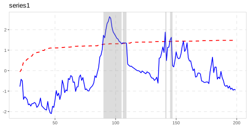
The other three are different. They carry the radf_obj class but build their statistic on gls_dfstat_grid() and do not call radf() directly. This function is a no-intercept, GLS-demeaned recursive Dickey-Fuller grid. It is fed the raw series for radf_tt(), the cumulated sign of the series for radf_sign(), and a recursively demeaned cumulated sign for radf_sign_dm().
The _cv() functions of all three return the time-varying boundaries badf_cv and bsadf_cv as well as the three scalar critical values, so datestamp() and autoplot() work on them. The bsadf that gls_dfstat_grid() returns is already the sup over all window starts at each point. This differs from radf_mc_cv(), which applies a cummax() across replicates because of the output shape of the base C++ engine. Here the boundary is the per-time-point quantile across replicates, the same construction radf_mc_cv() uses for its own bsadf_cv.
Each function is checked in three ways.
- The last row of
badf_cvis bit-identical toadf_cv, becauseadfis the last point ofbadfin every replicate. This is an exact identity, and it holds whichever series feedsgls_dfstat_grid(). - The empirical false-alarm rate under
H0is at or below the nominal 5% (radf_tt3.3%,radf_sign5.5%,radf_sign_dm3.5%, with n = 100 and minw = 20). - The detection power on an identical synthetic bubble is in the same range as the 16% of the established
radf()andradf_mc_cv()baseline, and it is neither suspiciously higher nor lower (radf_tt18%,radf_sign20%,radf_sign_dm8%). The sign-based tests give up power in exchange for invariance to heteroskedasticity, which is a documented finding of the source paper.
res <- radf_tt(y, minw = 20)
cv <- radf_tt_cv(n = 200, minw = 20)

summary(res, cv = cv)
#>
#> ── Summary (minw = 20, lag = 0) ────────── Time-Transformed MC (nboot = 2000) ──
#>
#> series1 :
#> # A tibble: 3 × 5
#>   stat   tstat  `90`  `95`  `99`
#>   <fct>  <dbl> <dbl> <dbl> <dbl>
#> 1 adf   -0.997 0.832  1.26  2.04
#> 2 sadf   3.27  2.32   2.66  3.32
#> 3 gsadf  4.23  3.26   3.65  4.38
datestamp(res, cv = cv)
#>
#> ── Datestamp (min_duration = 0) ───────────────────────── Time-Transformed MC ──
#>
#> series1 :
#>   Start Peak End Duration   Signal Ongoing
#> 1    21   38  89       68 negative   FALSE
#> 2   148  148 150        2 positive   FALSE
tidy(res, cv = cv)
#> # A tibble: 1 × 4
#>   id         adf  sadf gsadf
#>   <fct>    <dbl> <dbl> <dbl>
#> 1 series1 -0.997  3.27  4.23
autoplot(res, cv = cv)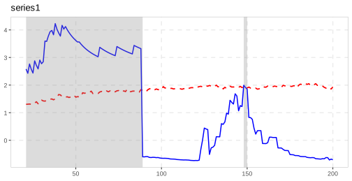
res <- radf_sign(y, minw = 20)
cv <- radf_sign_cv(n = 200, minw = 20)

summary(res, cv = cv)
#>
#> ── Summary (minw = 20, lag = 0) ──────────────── Sign-Based MC (nboot = 2000) ──
#>
#> series1 :
#> # A tibble: 3 × 5
#>   stat   tstat  `90`  `95`  `99`
#>   <fct>  <dbl> <dbl> <dbl> <dbl>
#> 1 adf   -0.293 0.932  1.35  2.14
#> 2 sadf   4.47  2.43   2.78  3.26
#> 3 gsadf  8.88  3.46   3.88  4.98
datestamp(res, cv = cv)
#>
#> ── Datestamp (min_duration = 0) ─────────────────────────────── Sign-Based MC ──
#>
#> series1 :
#>   Start Peak End Duration   Signal Ongoing
#> 1    84   84  85        1 positive   FALSE
#> 2    87  103 122       35 positive   FALSE
#> 3   123  123 124        1 positive   FALSE
tidy(res, cv = cv)
#> # A tibble: 1 × 4
#>   id         adf  sadf gsadf
#>   <fct>    <dbl> <dbl> <dbl>
#> 1 series1 -0.293  4.47  8.88
autoplot(res, cv = cv)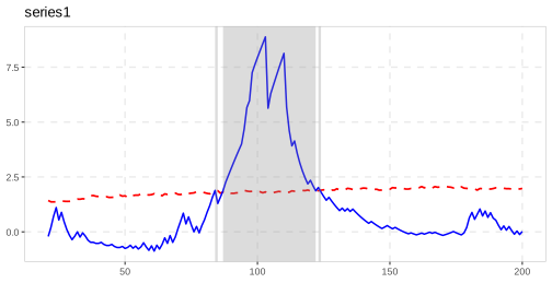
radf_sbz() is a fourth, separate case. It builds its statistic (supBZ) on wls_dfstat_grid(), a no-intercept recursive Dickey-Fuller grid weighted by WLS and kernel volatility, and not on gls_dfstat_grid(). The same fix applies for the same reason, since wls_dfstat_grid() already returns the full badf and bsadf path for each replicate. The wild bootstrap in radf_sbz_cv() is therefore built as the Monte Carlo simulation in radf_tt_cv() and radf_sign_cv() is, with a per-time-point quantile across replicates and no cummax() shortcut. We validated it in the same way. The last row of badf_cv is bit-identical to adf_cv, and the empirical false-alarm rate under H0 is 5.0% at a nominal 5% (n = 100, minw = 20, 200 replications). The test also rejects on a sufficiently strong deterministic explosive path. Its kernel-volatility weighting costs enough power, however, that it does not reject the series above at nboot = 100 to 200, where the bubble is the milder default of sim_psy1(). The same trade between power and robustness is documented for the supBZ leg of radf_sbz_union() below, so it is not new to this split.
res <- radf_sbz(y, minw = 20)
cv <- radf_sbz_cv(y, minw = 20, nboot = 200, seed = 1)

summary(res, cv = cv)
#>
#> ── Summary (minw = 20, lag = 0) ────────── Wild Bootstrap (SBZ) (nboot = 200) ──
#>
#> series1 :
#> # A tibble: 3 × 5
#>   stat  tstat  `90`  `95`  `99`
#>   <fct> <dbl> <dbl> <dbl> <dbl>
#> 1 adf   -1.39 0.825  1.13  1.61
#> 2 sadf   1.67 1.58   2.11  3.36
#> 3 gsadf  1.91 3.37   5.06  6.21
tidy(res, cv = cv)
#> # A tibble: 1 × 4
#>   id        adf  sadf gsadf
#>   <fct>   <dbl> <dbl> <dbl>
#> 1 series1 -1.39  1.67  1.91
datestamp() and autoplot() need at least one rejection to have anything to show, and they raise an error otherwise, as for any other radf_obj and radf_cv pair. The series above does not clear the supBZ threshold, so we repeat the volatility break with a stronger explosive regime that does not collapse (rho = 1.03 from t = 120 to the end of the sample):
y_strong <- sim_psy1(n = 200, te = 120, tf = 200, c = 0.03, alpha = 0, seed = 1,
                     e = sim_vol_break(199))

res2 <- radf_sbz(y_strong, minw = 20)
cv2 <- radf_sbz_cv(y_strong, minw = 20, nboot = 100, seed = 1)
datestamp(res2, cv = cv2)
#>
#> ── Datestamp (min_duration = 0) ──────────────────────── Wild Bootstrap (SBZ) ──
#>
#> series1 :
#>   Start Peak End Duration   Signal Ongoing
#> 1   128  129 130        2 positive   FALSE
#> 2   132  134 135        3 positive   FALSE
#> 3   172  200 200       29 positive    TRUE
autoplot(res2, cv = cv2)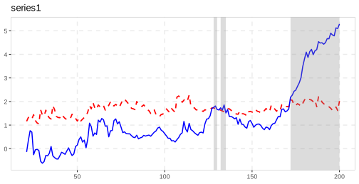
Own print() and autoplot(): everything else
The remaining 15 or so functions return their own class, with their own print() and autoplot() methods. They are lbi_test(), ssu_test(), quantile_test(), cobubble_test(), the dating_*() family, the monitor() and monitor_*() family (including monitor() itself, despite its ADF-family internals), contagion_reg(), radf_recovery(), rootstamp() and radf_sbz_union(). Their output does not fit the radf_obj shape: a dating table is not a per-series sup-statistic, and a monitoring alarm is not a critical value grid. Forcing them through summary(), datestamp() and tidy() would not close a documentation gap, so each is presented by its own methods, shown below.
rootstamp() needs one remark. The reference index and the workflow list in the README place it under Analysis, right after datestamp(), because that is its position in the sequence of steps (detect, date, measure the growth rate). That is a position in the workflow and not an S3-support tier. It has its own class with its own print() and autoplot() methods, like everything else in this section. See the dating and root inference page.
dating_hls(sim_data$psy1, trim = 0.05)
#>
#> ── dating_hls (n = 100, trim = 0.05) ───────────────────────────────────────────
#>
#>    series  model  origination  collapse  recovery
#>   series1      4           41        55        62

ssu_test(sim_data$psy1, sig_lvl = 95)
#>
#> ── ssu_test (SSU, n = 100, minw = 19, sig_lvl = 95%, crit = 3.3) ───────────────
#>
#>    series   sadf  detected
#>   series1  4.356      TRUE
autoplot(dating_hls(sim_data$psy1, trim = 0.05))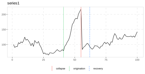
Summary
| Tier | Functions | summary() | datestamp() | tidy() | autoplot() |
|---|---|---|---|---|---|
| Full | radf(), radf_common(), radf_kp(), radf_tt(), radf_sign(), radf_sign_dm(), radf_sbz() | yes | yes | yes | yes |
| Standalone | everything else | own print() | — | — | own method |
Plotting with exuber
library(exuber)
library(ggplot2)
One autoplot() per object
Every result object in the package has an autoplot() method. The call is always autoplot(x), and what it draws depends on the class of x. Each method returns an ordinary ggplot object, so anything ggplot2 offers, such as themes, scales, extra layers and facet_*() arguments, can be added on top.
| What you have | What autoplot() draws |
|---|---|
radf() result (radf_obj) | Test statistic against the critical-value sequence, with one facet per series that rejects the null and the explosive episodes shaded |
datestamp() result (ds_radf) | Only the episodes, as one horizontal segment per series. This is the view for many series at once |
radf_*_distr() result (radf_distr) | The simulated null distribution of the ADF/SADF/GSADF statistics |
Any sim_*() series | The series itself |
monitor(), monitor_*() | Monitored statistic against its boundary, with markers for the end of training and for the alarm |
dating_*(), radf_recovery() | The series with vertical markers at the estimated break dates |
rootstamp() | Estimated root and its confidence interval per episode |
lbi_test(), quantile_test(), radf_sbz_union() | Statistic against critical value for each series |
The rest of this vignette covers the first three rows, which belong to the radf() workflow, and shows how to build your own plot from the tidied tables when the defaults do not fit. The other methods take no options beyond the object. They appear in their own vignettes (the real-time monitoring for bubbles page, the dating and root inference page and the dating and root inference page).
The radf() plot
We simulate four series, one from each of the classic bubble data generating processes in the package (see the simulating bubbles page), and estimate them with one lag. The critical values depend on (n, lag), so we simulate them once and pass them to every call, as in Getting started:
sims <- data.frame(
  psy1 = sim_psy1(100, seed = 1),
  psy2 = sim_psy2(100, seed = 2),
  evans = sim_evans(100, seed = 3),
  blan = sim_blan(100, seed = 4)
)
est <- radf(sims, lag = 1)
cv <- radf_mc_cv(100, lag = 1, seed = 1)autoplot(est, cv)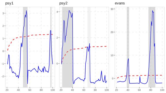
Only series that reject the null at the 5% level are drawn. The arguments of autoplot() itself control what is plotted:
# Every series, whether or not it rejects
autoplot(est, cv, nonrejected = TRUE)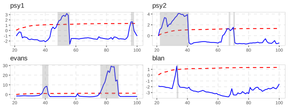
# A subset, by name or position; the SADF sequence instead of the BSADF one
autoplot(est, cv, select_series = c("psy1", "evans"), option = "sadf")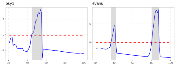
The shading of the explosive episodes is a geom_rect() layer. The shade_opt argument and the shade() helper control it, and shade_opt = NULL removes it:
autoplot(est, cv, select_series = "psy2",
         shade_opt = shade(fill = "pink", opacity = 0.3))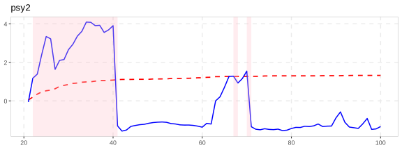
autoplot2() draws the series itself instead of the statistic, with the same shading. This is often easier to read for a non-technical audience. The method for datestamp() objects reduces each series to its episodes:
autoplot2(est, cv, select_series = "psy2")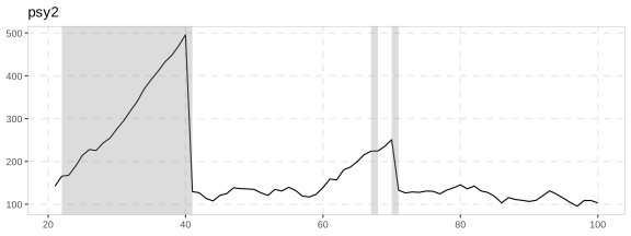
datestamp(est, cv) %>%
  autoplot()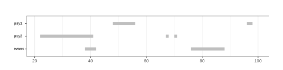
Changing the appearance
Colors, line types and themes are handled by ggplot2. autoplot() maps the statistic and the critical value to color, size and linetype, so the ggplot2 scale_*_manual() functions can override them. scale_exuber_manual() sets all three at once. theme_exuber() is the default theme of the package, and it is exported so that you can apply it to your own plots too:
autoplot(est, cv, select_series = "psy2") +
  scale_exuber_manual(color_values = c("grey40", "black"),
                      linetype_values = c(3, 1)) +
  theme_classic()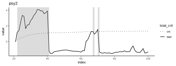
Arguments that autoplot() does not recognize are passed on to ggplot2::facet_wrap(), so scales = "free_y", ncol and labeller work directly. ?autoplot.radf_obj has a labeller example that renames the facets.
Building your own plot
When the default layout does not suit you, skip autoplot() and start from the table it is built on. augment_join() joins the full statistic sequences of a radf_obj with the critical-value sequences of a radf_cv. It returns one row per observation, series, statistic and significance level, which ggplot2 can use as it is:
joined <- augment_join(est, cv)
joined
#> # A tibble: 1,920 × 8
#>      key index id     data stat   tstat sig    crit
#>    <int> <dbl> <fct> <dbl> <fct>  <dbl> <fct> <dbl>
#>  1    21    21 psy1   126. badf  -1.05  90    -0.44
#>  2    22    22 psy1   132. badf  -0.630 90    -0.44
#>  3    23    23 psy1   137. badf  -0.289 90    -0.44
#>  4    24    24 psy1   138. badf  -0.350 90    -0.44
#>  5    25    25 psy1   124. badf  -1.41  90    -0.44
#>  6    26    26 psy1   129. badf  -1.23  90    -0.44
#>  7    27    27 psy1   128. badf  -1.28  90    -0.44
#>  8    28    28 psy1   127. badf  -1.36  90    -0.44
#>  9    29    29 psy1   117. badf  -1.68  90    -0.44
#> 10    30    30 psy1   114. badf  -1.77  90    -0.44
#> # ℹ 1,910 more rows
joined %>%
ggplot(aes(x = index)) +
geom_line(aes(y = tstat)) +
geom_line(aes(y = crit), linetype = 2) +
facet_grid(sig + stat ~ id, scales = "free_y") +
theme_exuber()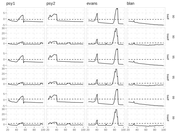
tidy_join() is the scalar counterpart, with one row per series and statistic, which is the table that summary() prints. Calling tidy() or augment() on either object alone returns the two halves before they are joined. the results, tidying and plotting page describes the full pipeline.
Distributions
The radf_*_distr() functions are the counterparts of the critical-value functions. They return the whole simulated null distribution instead of its quantiles, and they have their own autoplot() method:
distr <- radf_mc_distr(n = 100, nrep = 1000, seed = 1)
autoplot(distr)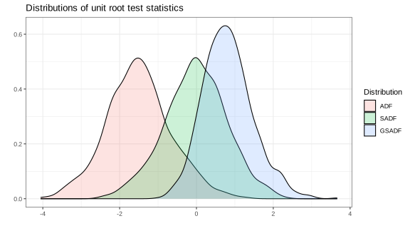
As elsewhere, tidy() returns the underlying table, so an empirical CDF or any other summary takes only a few lines of ggplot2:
distr %>%
  tidy() %>%
  tidyr::pivot_longer(everything(), names_to = "statistic") %>%
  ggplot(aes(value, color = statistic)) +
  stat_ecdf() +
  geom_hline(yintercept = 0.95, linetype = 2) +
  labs(title = "Empirical CDF of the null distributions", y = NULL) +
  theme_exuber()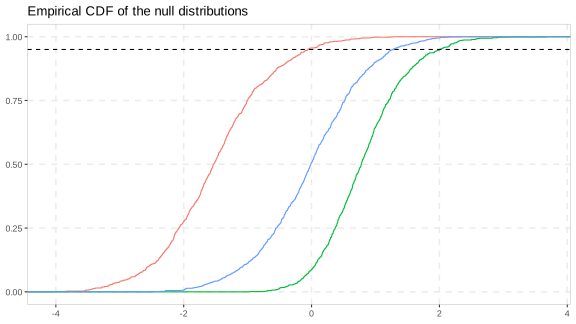
Which to reach for
- For a quick look at which series are explosive and when, use
autoplot(est, cv). Addnonrejected = TRUEto include the series that do not reject. - To show the series itself with the episodes shaded, for a non-technical reader, use
autoplot2(est, cv). - To show only the episodes of many series, use
autoplot(datestamp(est, cv)). - For cosmetic changes, keep
autoplot()and add ggplot2 layers, scales or a theme. Usescale_exuber_manual()to style the statistic and the critical value. - For a different layout altogether, build your own plot from
augment_join(est, cv).