Volatility-robustness tests

Volatility-Robust Alternatives to radf()

library(exuber)

The shared problem

Plain radf() assumes a constant innovation variance. Real series rarely have one, and when volatility varies over time the standard critical values no longer control the size of the test. exuber offers several fixes, and each takes a structurally different approach. Four of the five covered below (radf_sign(), radf_sign_dm(), radf_kp() and radf_sbz()) keep the radf_obj class and support summary(), datestamp(), tidy() and autoplot() in the same way as plain radf(). the results, tidying and plotting page shows how each plugs into the pipeline and how we validated it. radf_sbz_union() is the exception. It bundles the statistic of radf_sbz() and the classic supDF into one union-of-rejections call and has its own class, not radf_obj, so only its own print() and autoplot() apply. The time-deformation approach of radf_tt() has its own vignette, the volatility-robustness tests page, and this one covers the rest.

All of these functions target non-stationary volatility, meaning a permanent shift or trend in the unconditional innovation variance. They do not target stationary GARCH-type conditional heteroskedasticity, whose variance profile is asymptotically flat and leaves plain radf() with the correct size. The running example is therefore the sim_psy1() bubble driven by sim_vol_break() innovations, whose standard deviation triples half-way through the sample. This is the case in which plain radf() over-rejects the most:

y <- sim_psy1(n = 200, seed = 1, e = sim_vol_break(199))

Sign-based: radf_sign()

radf_sign() has full pipeline support. radf_sign_cv() computes the time-varying badf_cv and bsadf_cv boundary and not only the scalar critical values that summary() needs (see the results, tidying and plotting page for the validation):

res <- radf_sign(y, minw = 20)
cv <- radf_sign_cv(n = 200, minw = 20)
summary(res, cv = cv)
#> 
#> ── Summary (minw = 20, lag = 0) ──────────────── Sign-Based MC (nboot = 2000) ──
#> 
#> series1 :
#> # A tibble: 3 × 5
#>   stat   tstat  `90`  `95`  `99`
#>   <fct>  <dbl> <dbl> <dbl> <dbl>
#> 1 adf   -0.293 0.855  1.32  2.06
#> 2 sadf   4.47  2.34   2.70  3.43
#> 3 gsadf  8.88  3.51   3.91  4.92
datestamp(res, cv = cv)
#> 
#> ── Datestamp (min_duration = 0) ─────────────────────────────── Sign-Based MC ──
#> 
#> series1 :
#>   Start Peak End Duration   Signal Ongoing
#> 1    84   84  85        1 positive   FALSE
#> 2    87  103 122       35 positive   FALSE
#> 3   123  123 124        1 positive   FALSE

Kernel-purged: radf_kp()

radf_kp() purges volatility and then calls radf() unmodified, so it has full pipeline support in the simplest possible way. It needs no new critical-value code, and radf_mc_cv() applies as it is:

res_kp <- radf_kp(y, minw = 20)
cv_kp <- radf_mc_cv(n = attr(res_kp, "n"), minw = 20)
summary(res_kp, cv = cv_kp)
#> 
#> ── Summary (minw = 20, lag = 0) ────────────────── Monte Carlo (nboot = 1000) ──
#> 
#> series1 :
#> # A tibble: 3 × 5
#>   stat  tstat   `90`   `95`  `99`
#>   <fct> <dbl>  <dbl>  <dbl> <dbl>
#> 1 adf   -1.72 -0.470 -0.140 0.535
#> 2 sadf   1.50  1.07   1.37  1.90 
#> 3 gsadf  2.63  1.98   2.25  2.80

WLS + kernel volatility: radf_sbz()

radf_sbz() is a statistic function of its own, separate from the union test. radf_sbz_cv() computes the time-varying badf_cv and bsadf_cv boundary in the same way as radf_tt_cv() and radf_sign_cv() (see the results, tidying and plotting page for the validation), so it has full pipeline support:

res_sbz <- radf_sbz(y, minw = 20)
cv_sbz <- radf_sbz_cv(y, minw = 20, nboot = 200, seed = 1)
summary(res_sbz, cv = cv_sbz)
#> 
#> ── Summary (minw = 20, lag = 0) ────────── Wild Bootstrap (SBZ) (nboot = 200) ──
#> 
#> series1 :
#> # A tibble: 3 × 5
#>   stat  tstat  `90`  `95`  `99`
#>   <fct> <dbl> <dbl> <dbl> <dbl>
#> 1 adf   -1.39 0.825  1.13  1.61
#> 2 sadf   1.67 1.58   2.11  3.36
#> 3 gsadf  1.91 3.37   5.06  6.21

The kernel-volatility weighting that makes supBZ robust to heteroskedasticity costs some power relative to the other tests. The default bubble of sim_psy1() is mild (30 periods at rho = 1 + 200^-0.6, then a collapse). It does not clear the 95% critical value of supBZ here, although every other test above rejects on the same series. A stronger bubble that does not collapse (rho = 1.03 from t = 120 to the end of the sample, on the same volatility break) does clear it:

y_strong <- sim_psy1(n = 200, te = 120, tf = 200, c = 0.03, alpha = 0, seed = 1,
                     e = sim_vol_break(199))
res_sbz2 <- radf_sbz(y_strong, minw = 20)
cv_sbz2 <- radf_sbz_cv(y_strong, minw = 20, nboot = 200, seed = 1)
summary(res_sbz2, cv = cv_sbz2)
#> 
#> ── Summary (minw = 20, lag = 0) ────────── Wild Bootstrap (SBZ) (nboot = 200) ──
#> 
#> series1 :
#> # A tibble: 3 × 5
#>   stat  tstat  `90`  `95`  `99`
#>   <fct> <dbl> <dbl> <dbl> <dbl>
#> 1 adf    4.83 0.948  1.65  2.65
#> 2 sadf   4.83 2.24   2.49  3.26
#> 3 gsadf  5.29 2.77   3.00  3.58
datestamp(res_sbz2, cv = cv_sbz2)
#> 
#> ── Datestamp (min_duration = 0) ──────────────────────── Wild Bootstrap (SBZ) ──
#> 
#> series1 :
#>   Start Peak End Duration   Signal Ongoing
#> 1   129  129 130        1 positive   FALSE
#> 2   132  132 133        1 positive   FALSE
#> 3   134  134 135        1 positive   FALSE
#> 4   172  200 200       29 positive    TRUE

This is the same trade-off that radf_sbz_union(), below, hedges against by combining supBZ with the classic supDF.

Union-of-rejections: radf_sbz_union()

radf_sbz_union(y, nboot = 200, seed = 1)
#> 
#> ── radf_sbz_union (minw = 27, nboot = 200) ─────────────────────────────────────
#> 
#>    series  supDF  supBZ      U  p_supDF  p_supBZ    p_U
#>   series1  9.329   1.67  9.329        0    0.085  0.005

supDF is the classic PWY statistic, and supBZ is the WLS-weighted version that radf_sbz() also returns on its own. U is their union. Each statistic has its own bootstrap p-value, so one can flag a series without the other. Here supDF rejects, supBZ does not, and the union U follows supDF. The value of U is defined with a bootstrap-derived scaling ratio between supDF and supBZ, and its size guarantee requires that the supDF and supBZ bootstrap draws come from the same resampled series in each replicate. For both reasons radf_sbz_union() cannot be reconstructed by calling radf_sbz_cv() and plain radf_wb_cv() separately. It stays a single bundled call with its own class and is not a radf_obj.

Which to reach for

• If you want exact invariance to any heteroskedasticity pattern with no bootstrap, use radf_sign(). Use radf_sign_dm() if a level shift, and not only volatility, is a concern. Both have full pipeline support.
• If you want to stay closest to plain radf() with no new critical-value code, use radf_kp().
• If you want the efficiency gain from WLS together with full datestamp() and autoplot() support, use radf_sbz() with radf_sbz_cv().
• If you want to hedge between the classic and the WLS-weighted statistics on the same series and do not need datestamp() or autoplot(), use radf_sbz_union(). It is the only function in this group without pipeline support, because U bundles both statistics and their scalar joint critical value in one call and does not return a radf_obj.
• If volatility is the main concern and you prefer a time-deformation approach without a bootstrap, use radf_tt() (see the volatility-robustness tests page).
• If the volatility is unknown or complex and a bootstrap is acceptable, radf_wb_cv() remains the general-purpose choice.

Time-Transformed Test (STADF/GSTADF)

library(exuber)

Why another test

radf(), the classic PSY GSADF test, assumes that the innovation variance is constant. Real financial series usually do not have constant volatility. Harvey, Leybourne, Sollis & Taylor (2016) show that when volatility changes over time, the standard critical values of radf() no longer control the size of the test. radf_wb_cv() addresses this in exuber with a wild bootstrap.

radf_tt() implements a different fix that needs no bootstrap, from Kurozumi, Skrobotov & Tsarev (2024, Journal of Financial Econometrics). Instead of resampling, it time-deforms the series using a nonparametric estimate of its variance profile, so that under the null the deformed series behaves like a random walk with constant volatility. The null distribution of the resulting statistic is then the same pivotal distribution as under homoskedasticity. Ordinary asymptotic critical values therefore apply, with no bootstrap and no resimulation for each dataset.

Basic usage

radf_tt() targets non-stationary volatility, meaning a permanent shift or trend in the unconditional innovation variance, which is the setting of the simulations in Kurozumi, Skrobotov & Tsarev. It does not target stationary conditional heteroskedasticity such as GARCH. In that case the variance profile is asymptotically flat, the time deformation is close to the identity, and plain radf() already has the correct size. sim_vol_break() generates innovations with a permanent volatility shift, and the e argument of sim_psy1() passes them into the PSY bubble process. Here the innovation standard deviation triples half-way through the sample:

y <- sim_psy1(n = 200, seed = 1, e = sim_vol_break(199))
res <- radf_tt(y)
res
#> 
#> ── radf_tt (minw = 27, kernel = uniform) ───────────────────────────────────────
#> 
#>    series      adf   sadf  gsadf
#>   series1  -0.9972  3.275  4.165

radf_tt_cv() returns the matching pivotal asymptotic critical values. The null distribution does not depend on the volatility path, so one call with a large n approximates the whole family of cases. radf_wb_cv(), in contrast, runs a separate bootstrap for each dataset:

cv <- radf_tt_cv(n = 300, minw = 30, nrep = 1000, seed = 1)
cv$gsadf_cv
#>      90%      95%      99% 
#> 3.248911 3.584415 4.246916

What is estimated

radf_tt() works in three steps.

1. It estimates the time-varying AR(1) coefficient with a local kernel regression. From the truncated residuals it builds a monotone variance profile eta_hat(s), with s in [0, 1].
2. It inverts the profile and uses the inverse to resample and time-deform the series.
3. It computes a recursive sup-ADF statistic (GLS-demeaned, with no intercept) on the deformed series. This belongs to the same family of statistics as radf(), but it needs no fitted intercept, which matches the derivation in the paper.

You can adjust kernel ("uniform", the choice of the paper, or "gaussian") and h, the bandwidth. The default for h is a fixed plug-in value and not the full cross-validation search of the paper. The package’s enhancement notes explain why we weighed cost against benefit this way.

Verifying against the paper

Footnote 4 of Kurozumi, Skrobotov & Tsarev gives published asymptotic critical values for minw/n = 0.1: (2.319, 2.626, 3.223) at the 10%, 5% and 1% levels. They apply to the STADF statistic, the single-sup case with r1 = 0. The test suite of exuber (tests/testthat/test-tt.R) reproduces them with the Monte Carlo in radf_tt_cv() and checks that they fall within the Monte Carlo and finite-sample tolerance of the published numbers.

Dating and plotting a detected bubble

radf_tt() returns the same radf_obj class as radf(). radf_tt_cv() also computes the full time-varying boundary that dating and plotting need, and not only the summary-level critical values. The usual pipeline therefore works unchanged:

res <- radf_tt(y, minw = 20)
cv <- radf_tt_cv(n = 200, minw = 20)

datestamp(res, cv = cv)
#> 
#> ── Datestamp (min_duration = 0) ───────────────────────── Time-Transformed MC ──
#> 
#> series1 :
#>   Start Peak End Duration   Signal Ongoing
#> 1    21   38  89       68 negative   FALSE
#> 2   148  148 150        2 positive   FALSE
autoplot(res, cv = cv)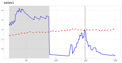

the results, tidying and plotting page explains which other exuber functions work with this pipeline and which do not.