 exuber
library(exuber)
library(ggplot2)
What the sim_*() family is for
Every test in the package is calibrated and validated on simulated data. The same data generating processes are exported, so you can check the size of a test under a null you choose, check its power against a bubble you choose, or see what a test does to a series whose true break dates you know. There are three kinds:
| Kind | Functions | Returns |
|---|---|---|
| Bubble processes | sim_psy1(), sim_psy2(), sim_ps1(), sim_blan(), sim_evans(), sim_div(), sim_tree(), sim_mar(), sim_msbubble(), sim_falsebubble() | One series (class "sim", plots with autoplot()) |
| Innovation generators | sim_innov(), sim_vol_garch(), sim_vol_break(), sim_vol_cir(), sim_vol_sv(), sim_fi() | One series of shocks, to feed into a bubble process through its e argument |
| Multi-series processes | sim_common(), sim_coexplosive() | A data.frame, one column per series |
The package also bundles sim_data and sim_data_wdate, two data.frames with five of the classic series, without and with a date column, which the examples use throughout.
Every function takes a seed argument, so a series is reproducible without a surrounding set.seed(). The bubble processes take the break dates (te, tf and so on) as arguments, so the truth you test against is explicit.
The bubble processes fall into two families. sim_psy1(), sim_psy2() and sim_ps1() are the regime processes of Phillips, Shi & Yu (2015) and Phillips & Shi (2018). They have a unit root, then an explosive AR(1) between fixed dates, then a collapse and a return to a unit root. Papers in this literature use this design to study size and power. sim_blan(), sim_evans(), sim_tree(), sim_mar() and sim_msbubble() are rational bubble models. The explosive behavior and the collapse are stochastic, driven by a probability that the bubble bursts in each period and not by fixed dates. The periodically collapsing bubble of sim_evans() is the one that the GSADF test of PSY was designed to detect and that the earlier tests it replaced could not.
The PSY experiment
PSY validate the GSADF test on a price built from Lucas-model fundamentals plus an Evans (1991) bubble. sim_div() produces the fundamental price from a random walk with drift in dividends, using by default the S&P 500 parameterization of West (1988). sim_evans() produces the bubble term, and a scaling factor kappa sets how much of the price the bubble accounts for:
n <- 200
pf <- sim_div(n, seed = 1)          # fundamental price
pb <- sim_evans(n, seed = 3)        # periodically collapsing bubble
p <- pf + 20 * pb # kappa = 20data.frame(index = seq_len(n), fundamental = pf, price = p) %>%
tidyr::pivot_longer(-index) %>%
ggplot(aes(index, value, color = name)) +
geom_line() +
labs(y = NULL, x = NULL, color = NULL) +
theme_exuber()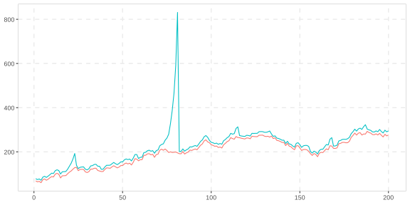
radf() should find the episodes:
cv <- radf_mc_cv(n, seed = 1)
datestamp(radf(p), cv)
#>
#> ── Datestamp (min_duration = 0) ───────────────────────────────── Monte Carlo ──
#>
#> series1 :
#>   Start Peak End Duration   Signal Ongoing
#> 1    75   81  82        7 positive   FALSE
Plotting a simulated series
Each series has an autoplot() method:
sim_psy2(100, seed = 1) %>%
  autoplot()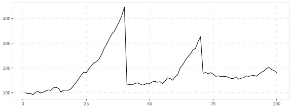
Several series can be collected in a data.frame, which is also what radf() takes, so the same object serves both purposes:
sims <- data.frame(
  psy1 = sim_psy1(100, seed = 1),
  psy2 = sim_psy2(100, seed = 2),
  evans = sim_evans(100, seed = 3),
  blan = sim_blan(100, seed = 4)
)
sims %>%
dplyr::mutate(dplyr::across(dplyr::everything(), as.numeric), index = dplyr::row_number()) %>%
tidyr::pivot_longer(-index, names_to = "id") %>%
ggplot(aes(index, value)) +
geom_line() +
facet_wrap(~id, scales = "free_y") +
theme_exuber()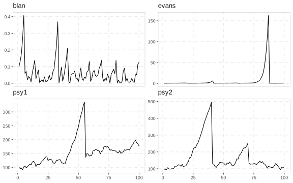
Swapping the innovations
By default the regime processes are driven by i.i.d. Gaussian shocks. Every bubble process also accepts a vector of innovations through e, and the innovation generators exist to supply it. They produce heavy-tailed or skewed marginals (sim_innov()), conditional heteroskedasticity (sim_vol_garch()), a one-off variance break (sim_vol_break()), stochastic volatility (sim_vol_cir() and sim_vol_sv()) or long memory (sim_fi()). The bubble dates stay where you put them and only the noise changes. This is how the volatility-robustness tests page compares the volatility-robust tests with plain radf() on an equal footing:
# Same bubble, same seed, volatility tripling half-way through the sample
sim_psy1(n = 200, seed = 1, e = sim_vol_break(199, seed = 1)) %>%
  autoplot()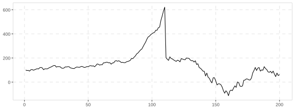
The innovation vector is one element shorter than n because the first observation is the starting value and not a shock.
Multi-series processes
sim_common() draws n_series series that share one latent bubble plus idiosyncratic noise, which is the design behind the panel test radf_common(). sim_coexplosive() draws a pair in which y is a linear function of a possibly lagged explosive x. This is the design behind cobubble_test() and contagion_reg() (see the multivariate bubble tests page):
head(sim_common(n_series = 3, n = 100, seed = 1))
#>   series_1 series_2 series_3
#> 1 63.51506 156.4806 53.64832
#> 2 60.82614 150.0373 51.29328
#> 3 61.68536 151.9221 52.08866
#> 4 57.95947 143.0566 48.83047
#> 5 65.01851 160.0944 54.52820
#> 6 66.25556 163.4051 55.81010
head(sim_coexplosive(n = 100, lag = 2, seed = 1))
#>           x         y
#> 1 100.00000        NA
#> 2  95.74638        NA
#> 3  96.99332 100.28597
#> 4  91.31940  89.56122
#> 5 102.15136  98.06633
#> 6 104.38871  86.87477
Which to reach for
- To study the size or power of a test against a bubble with known dates, use
sim_psy1()(one episode),sim_psy2()(two episodes) orsim_ps1()(one episode with a distinct collapse regime, the design that thedating_*()estimators assume). - For a rational bubble that collapses stochastically, use
sim_evans()alone or on top ofsim_div()fundamentals, as in PSY.sim_blan()gives the Blanchard version, andsim_tree(),sim_mar()andsim_msbubble()give the newer ones. - For a null that looks like a bubble but is not one, use
sim_falsebubble(). - For non-Gaussian or heteroskedastic shocks under any of these processes, build the shocks with an innovation generator and pass them as
e. - For several series, use
sim_common()for a shared bubble,sim_coexplosive()for a linked pair, or adata.frameof independent draws.