 exuber
Multivariate / panel bubble tests
Bubble Contagion Regression (Greenaway-McGrevy & Phillips 2016)
contagion_reg
Replication record →
contagion_reg(
  y,
  core,
  S = NULL,
  d = 0L,
  h = NULL,
  r_grid = seq(0, 1, length.out = 100)
)
contagion_reg estimates the time-varying contagion coefficient of Greenaway-McGrevy & Phillips (2016). It computes a fixed-window rolling AR(1) coefficient sequence for a "core" series and for a "satellite" series y and relates them with a functional (Nadaraya-Watson kernel) regression at a chosen delay d. The coefficient shows how strongly, and how it varies over time, the local persistence of the core series transmits to y, d periods later.
Arguments
| y | Satellite (dependent) series, a numeric vector. |
| core | Core (reference) series, a numeric vector of the same length as
y. |
| S | Fixed rolling-window width for the AR(1) coefficient sequence (default
floor(0.33 * length(y)), the choice of the paper). |
| d | Non-negative integer delay (default 0). |
| h | Bandwidth for the Nadaraya-Watson regression. The default NULL
selects it by leave-one-out cross-validation (eq. 7). |
| r_grid | Evaluation points for the time-varying coefficient, as fractions
of the sample (default seq(0, 1, length.out = 100)). |
Value
An object of class contagion_reg_obj: a list with the fixed-window AR(1) coefficient sequences (beta_core and beta_j), the selected or supplied bandwidth (h) and the estimated time-varying contagion coefficient (delta2, aligned with r_grid).
Details
This is a minimal subset of the procedure in the paper. It contains the fixed-window AR(1) coefficient sequence (their eq. 1), the Nadaraya-Watson regression at a single supplied d (eq. 6) and leave-one-out cross-validated bandwidth selection (eq. 7). Their eq. 8, the automatic search over d, is not implemented. If you need a search, call contagion_reg once for each candidate d and compare the fit.
The paper performs no formal inference on the contagion coefficient itself, with no confidence bands and no hypothesis test. As in the paper, this function is a tool for point estimation and visualization and not a test.
Status
[Experimental]
Examples
These examples are copied from the package's own documentation and are run by R CMD check on every release.
The printed output (after #>) and the plots were produced by running them against the current package source.
# A co-explosive pair: the AR coefficient of y follows that of x almost one for one
xy <- sim_coexplosive(n = 100, seed = 123)
res <- contagion_reg(xy$y, xy$x, d = 0L)
print(res)
#>
#> ── contagion_reg (n = 100, S = 33, d = 0, h = 0.6567) ──────────────────────────
#>
#> delta_2(r) range: [0.948, 0.965]

# Plot the estimated time-varying contagion coefficient
autoplot(res)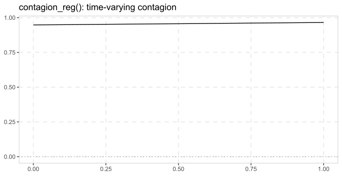
# Compare a one-period lead (d = 1) with the contemporaneous case
res_d1 <- contagion_reg(xy$y, xy$x, d = 1L)
autoplot(res) +
  ggplot2::geom_line(data = data.frame(r = res_d1$r_grid, delta2 = res_d1$delta2),
    ggplot2::aes(r, delta2), color = "red", inherit.aes = FALSE)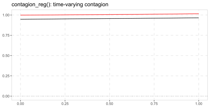
See also
cobubble_test for a different, symmetric bivariate bubble relationship that uses a hypothesis test.
Other multivariate: cobubble_test(), radf_common()
References
Greenaway-McGrevy, R., & Phillips, P. C. B. (2016). Hot property in New Zealand: Empirical evidence of housing bubbles in the metropolitan centres. New Zealand Economic Papers, 50(1), 88-113.