Analysis

Date-stamping periods of mildly explosive behavior

Also: datestamp.radf_obj

datestamp

datestamp(object, cv = NULL, min_duration = 0L, ...)

datestamp(
  object,
  cv = NULL,
  min_duration = 0L,
  sig_lvl = 95,
  option = c("gsadf", "sadf", "svadf"),
  nonrejected = FALSE,
  ...
)

Computes the origination, termination and duration of the episodes in which a time series shows explosive dynamics.

Arguments

object	An object of class `obj`.
cv	An object of class `cv`.
min_duration	The minimum duration of an explosive period for it to be reported (default = 0).
...	Further arguments passed to methods.
sig_lvl	Significance level, one of 90, 95 or 99. It is ignored when `option = "svadf"`.
option	One of `"gsadf"` or `"sadf"`, which date episodes (PWY/PSY) against the critical values in `cv`, or `"svadf"`, the SV-ADF asymmetric-threshold dating of Sarkar & Wells (2026). The `"svadf"` option compares the `badf` sequence of `radf()` with two closed-form thresholds that depend only on the sample size, `log(t)/10` for origination and `log(t)/2` for collapse, so it needs no `cv`. See Caveats.
nonrejected	logical. Whether to apply the datestamping technique to the series that do not reject the null hypothesis. It is ignored when `option = "svadf"`.

Value

A table with the following columns:

Start:
Peak:
End:
Duration:
Signal:
Ongoing:

A list with the estimated origination and termination dates of the episodes of explosive behavior and their duration.

Details

datestamp also stores a vector that takes the value 1 when there is a period of explosive behavior and 0 otherwise. You can use it as a dummy variable for the occurrence of exuberance.

Caveats

option = "svadf": [Experimental] Sarkar & Wells (2026) is a preprint that has not been peer reviewed, which is a weaker standard of evidence than for every other source this package implements. The function emits the same note as a message when you call it with this option. It detects at most one origination and collapse pair per series, as the procedure of the paper does, and it does not find every recurring episode as "gsadf" and "sadf" do.

Examples

These examples are copied from the package's own documentation and are run by R CMD check on every release. The printed output (after #>) and the plots were produced by running them against the current package source.

rsim_data <- radf(sim_data)

# SV-ADF asymmetric-threshold dating (no critical values needed)
datestamp(rsim_data, option = "svadf")
#> Experimental. Sarkar & Wells (2026) is a non-peer-reviewed preprint; see ?datestamp, Caveats section.
#> 
#> ── Datestamp (min_duration = 0) ──────────────── SV-ADF (Sarkar & Wells 2026) ──
#> 
#> ℹ Experimental. Sarkar & Wells (2026) is a non-peer-reviewed preprint; see ?datestamp, Caveats section.
#> 
#> psy1 :
#>   Start Peak End Duration   Signal Ongoing
#> 1    48   48  49        1 positive   FALSE
#> 
#> psy2 :
#>   Start Peak End Duration   Signal Ongoing
#> 1    23   23  24        1 positive   FALSE
#> 
#> evans :
#>   Start Peak End Duration   Signal Ongoing
#> 1    20   20  21        1 positive   FALSE
#> 
#> div :
#>   Start Peak End Duration   Signal Ongoing
#> 1    22   22  23        1 positive   FALSE
#> 
#> blan :
#>   Start Peak End Duration   Signal Ongoing
#> 1    35   36  37        2 positive   FALSE

# The default `cv` is fetched from the shared critical-value store
# (network on first use); pass `cv = radf_mc_cv(nrow(sim_data))` to stay offline
ds_data <- datestamp(rsim_data)
#> Using precomputed critical values for `cv`.
ds_data
#> 
#> ── Datestamp (min_duration = 0) ───────────────────────────────── Monte Carlo ──
#> 
#> psy1 :
#>   Start Peak End Duration   Signal Ongoing
#> 1    44   48  56       12 positive   FALSE
#> 
#> psy2 :
#>   Start Peak End Duration   Signal Ongoing
#> 1    23   40  41       18 positive   FALSE
#> 2    62   70  71        9 positive   FALSE
#> 
#> evans :
#>   Start Peak End Duration   Signal Ongoing
#> 1    20   20  21        1 positive   FALSE
#> 2    44   44  45        1 positive   FALSE
#> 3    66   67  68        2 positive   FALSE
#> 
#> blan :
#>   Start Peak End Duration   Signal Ongoing
#> 1    34   36  37        3 positive   FALSE
#> 2    84   86  87        3 positive   FALSE

# Choose minimum window
datestamp(rsim_data, min_duration = psy_ds(nrow(sim_data)))
#> Using precomputed critical values for `cv`.
#> 
#> ── Datestamp (min_duration = 5) ───────────────────────────────── Monte Carlo ──
#> 
#> psy1 :
#>   Start Peak End Duration   Signal Ongoing
#> 1    44   48  56       12 positive   FALSE
#> 
#> psy2 :
#>   Start Peak End Duration   Signal Ongoing
#> 1    23   40  41       18 positive   FALSE
#> 2    62   70  71        9 positive   FALSE

autoplot(ds_data)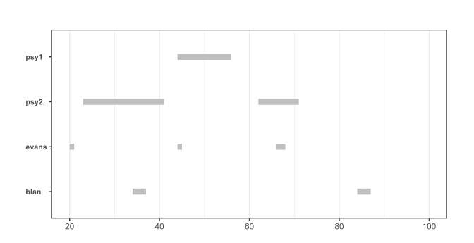

References

Phillips, P. C. B., Shi, S., & Yu, J. (2015). Testing for Multiple Bubbles: Historical Episodes of Exuberance and Collapse in the S&P 500. International Economic Review, 56(4), 1043-1078. 10.1111/iere.12132

Sarkar, A., & Wells, M. T. (2026). Is there an AI bubble? Robust date-stamping for periods of exuberance. arXiv:2604.12062.