 exuber
Analysis
Confidence Interval and Doubling Time for an Explosive Root
Also: rootstamp.default, rootstamp.radf_obj
rootstamp rootstamp(object, ...)
rootstamp(object, sig_lvl = 95, type = c("normal", "cauchy"), ...)
rootstamp(object, ds, sig_lvl = 95, type = c("normal", "cauchy"), ...)Fits a no-intercept AR(1) regression (Phillips & Magdalinos 2007, who omit the intercept in their eq. 58 "to exclude the presence of a deterministically explosive component") and reports together with a confidence interval and the implied doubling time , which is the number of periods the series needs to double in magnitude at the estimated growth rate.
Arguments
| object | For the default method, a numeric vector with the sub-sample to
fit, already sliced to the episode of interest. For the radf_obj method,
the radf_obj on which ds was computed. |
| ... | Further arguments passed to methods. |
| sig_lvl | Confidence level of the interval on the 0 to 100 scale used
throughout the package (default 95). Any value in [50, 100) is
allowed. |
| type | "normal" (default) for the normal-t interval of Guo, Sun &
Wang, or "cauchy" for the fixed-root Cauchy interval of Phillips &
Magdalinos. |
| ds | (radf_obj method only) A datestamp result
computed on object. Root inference on a very short episode is
statistically meaningless. Set min_duration in that
datestamp call to exclude episodes that are too short for reliable
root inference, because this method does not decide what counts as too short. |
Value
The default method returns a rootstamp_est object, which is a list with rho, se, t_stat, n, rho_ci, doubling_time and doubling_time_ci and has its own print() method.
The radf_obj method returns a rootstamp_episodes object, which is a named list with one element for each series in ds. Each element is a data frame with one row for each datestamped episode and the columns Start, End, rho, rho_lower, rho_upper, doubling_time, doubling_time_lower and doubling_time_upper. The object has its own print() method. The panel sieve-bootstrap case has a ds entry named "panel" that corresponds to no single series, and it is dropped with a warning.
Details
Guo, Sun & Wang (2019) show that the ordinary t-statistic for , estimated by OLS with no intercept, is asymptotically standard normal under i.i.d. errors, and also under weakly dependent errors when a HAC standard error is used. This differs from the classical stationary and unit-root cases. An ordinary-looking Wald interval, , is therefore asymptotically valid here even though . The interval has the same form as a classical normal-theory interval, which would be invalid for an explosive root, but the justification is different: it rests on the explosive-root central limit theorem of Guo, Sun & Wang and not on the classical stationary one.
type = "cauchy" instead uses the fixed-root result of Phillips & Magdalinos (2007, their eq. 27, which restates White 1958). For an explosive root that does not drift, converges to a standard Cauchy variate. We replace the unknown in the normalization with , as is usual for this kind of self-normalized pivot, and obtain , where is a standard-Cauchy quantile. This interval assumes a fixed explosive root, with no drift and no unknown localizing rate. When that assumption is in doubt, the default "normal" type is safer, because the result of Guo, Sun & Wang allows for drift and weak dependence.
There are two methods, for two different starting points:
- Default:
objectis a numeric vector, the sub-sample to fit. It can be an episode that you sliced out by hand or by position from adatestampresult (y[from:to]). The method fits the sub-sample once and returns one confidence interval. -
radf_obj:objectis theradf_objon which adatestampresultdswas computed. The method runs the default method once for each datestamped episode of each series and slices the data ofobjectitself, so no manual loop is needed.
Status
[Experimental]
Examples
These examples are copied from the package's own documentation and are run by R CMD check on every release.
The printed output (after #>) and the plots were produced by running them against the current package source.
# The martingale-to-explosive process of sim_psy1(), explosive through the sample end
y <- sim_psy1(n = 100, te = 60, tf = 100, seed = 2026)

r <- radf(y, minw = 20)
cv <- radf_mc_cv(length(y), minw = 20, nrep = 300, seed = 4)
ds <- datestamp(r, cv = cv, min_duration = 3)

# default method: one episode, sliced by hand
ep <- y[ds[["series1"]]$Start[1]:ds[["series1"]]$End[1]]
fit <- rootstamp(ep) # recovers the DGP's explosive AR coefficient
fit
#>
#> ── rootstamp (n = 22, sig_lvl = 95%, type = normal) ────────────────────────────
#>
#>     rho        se  t_stat  rho_lower  rho_upper  doubling_time  dt_lower
#>   1.059  0.005279   11.17      1.049      1.069           12.1     10.34
#>   dt_upper
#>       14.6
rootstamp(ep, type = "cauchy")
#>
#> ── rootstamp (n = 22, sig_lvl = 95%, type = cauchy) ────────────────────────────
#>
#>     rho        se  t_stat  rho_lower  rho_upper  doubling_time  dt_lower
#>   1.059  0.005279   11.17     0.6216      1.496           12.1      1.72
#>   dt_upper
#>     -1.458

# Plot the episode with the fitted explosive-root path overlaid
autoplot(fit)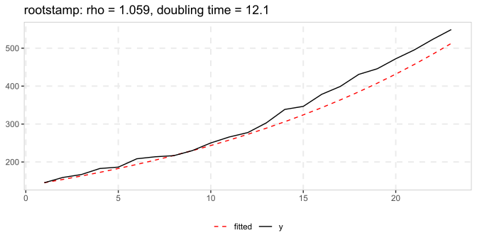
# radf_obj method: every datestamped episode at once
res_all <- rootstamp(r, ds)
res_all
#>
#> ── rootstamp (sig_lvl = 95%, type = normal) ────────────────────────────────────
#>
#> series1 :
#>   Start End   rho rho_lower rho_upper doubling_time doubling_time_lower
#> 1    78 100 1.059     1.049     1.069          12.1               10.34
#>   doubling_time_upper
#> 1                14.6

# Plot the estimated rho (with its CI) for every episode
autoplot(res_all)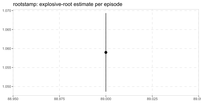
See also
Other dating: dating_hls(), dating_hlw(), dating_knp(), dating_pdc(), radf_recovery()
References
Guo, G., Sun, Y., & Wang, S. (2019). Testing for moderate explosiveness. The Econometrics Journal, 22(3), 279-303.
Phillips, P. C. B., & Magdalinos, T. (2007). Limit theory for moderate deviations from a unit root. Journal of Econometrics, 136(1), 115-130.