Recursive Augmented Dickey-Fuller

Summarizing radf models

summary.radf_obj

summary(object, cv = NULL, ...)

summary method for radf models, which consist of a radf_obj and a radf_cv.

Arguments

object	An object of class `radf_obj`. The output of `radf`.
cv	An object of class `radf_cv`. The output of `radf_mc_cv`, `radf_wb_cv` or `radf_sb_cv`.
...	Further arguments passed to methods. Not used.

Value

A list of summary statistics, which includes the estimated ADF, SADF and GSADF test statistics and the corresponding critical values.

Examples

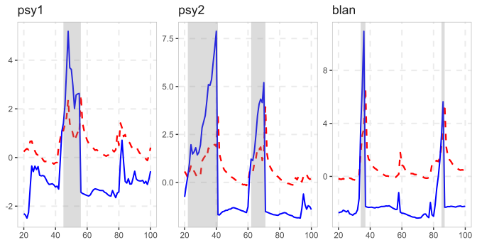
These examples are copied from the package's own documentation and are run by R CMD check on every release. The printed output (after #>) and the plots were produced by running them against the current package source.

# Simulate bubble processes, compute the test statistics and critical values
rsim_data <- radf(sim_data)

# Summary, diagnostics and datestamp (default)
summary(rsim_data)
#> Using precomputed critical values for `cv`.
#> 
#> ── Summary (minw = 19, lag = 0) ────────────────── Monte Carlo (nboot = 2000) ──
#> 
#> psy1 :
#> # A tibble: 3 × 5
#>   stat  tstat   `90`    `95`  `99`
#>   <fct> <dbl>  <dbl>   <dbl> <dbl>
#> 1 adf   -2.46 -0.412 -0.0178 0.644
#> 2 sadf   1.95  0.965  1.25   1.77 
#> 3 gsadf  5.19  1.65   1.93   2.60 
#> 
#> psy2 :
#> # A tibble: 3 × 5
#>   stat  tstat   `90`    `95`  `99`
#>   <fct> <dbl>  <dbl>   <dbl> <dbl>
#> 1 adf   -2.86 -0.412 -0.0178 0.644
#> 2 sadf   7.88  0.965  1.25   1.77 
#> 3 gsadf  7.88  1.65   1.93   2.60 
#> 
#> evans :
#> # A tibble: 3 × 5
#>   stat  tstat   `90`    `95`  `99`
#>   <fct> <dbl>  <dbl>   <dbl> <dbl>
#> 1 adf   -5.83 -0.412 -0.0178 0.644
#> 2 sadf   5.28  0.965  1.25   1.77 
#> 3 gsadf  5.99  1.65   1.93   2.60 
#> 
#> div :
#> # A tibble: 3 × 5
#>   stat  tstat   `90`    `95`  `99`
#>   <fct> <dbl>  <dbl>   <dbl> <dbl>
#> 1 adf   -1.95 -0.412 -0.0178 0.644
#> 2 sadf   1.11  0.965  1.25   1.77 
#> 3 gsadf  1.34  1.65   1.93   2.60 
#> 
#> blan :
#> # A tibble: 3 × 5
#>   stat  tstat   `90`    `95`  `99`
#>   <fct> <dbl>  <dbl>   <dbl> <dbl>
#> 1 adf   -5.15 -0.412 -0.0178 0.644
#> 2 sadf   3.93  0.965  1.25   1.77 
#> 3 gsadf 11.0   1.65   1.93   2.60

# Summary, diagnostics and datestamp (wild bootstrap critical values)

wb <- radf_wb_cv(sim_data)

summary(rsim_data, cv = wb)
#> 
#> ── Summary (minw = 19, lag = 0) ──────────────── Wild Bootstrap (nboot = 500) ──
#> 
#> psy1 :
#> # A tibble: 3 × 5
#>   stat  tstat   `90`   `95`   `99`
#>   <fct> <dbl>  <dbl>  <dbl>  <dbl>
#> 1 adf   -2.46 -0.596 -0.362 0.0523
#> 2 sadf   1.95  1.51   1.97  2.87  
#> 3 gsadf  5.19  2.80   3.34  4.35  
#> 
#> psy2 :
#> # A tibble: 3 × 5
#>   stat  tstat   `90`   `95`   `99`
#>   <fct> <dbl>  <dbl>  <dbl>  <dbl>
#> 1 adf   -2.86 -0.629 -0.530 -0.251
#> 2 sadf   7.88  3.07   3.88   5.59 
#> 3 gsadf  7.88  4.00   4.68   5.98 
#> 
#> evans :
#> # A tibble: 3 × 5
#>   stat  tstat   `90`   `95`    `99`
#>   <fct> <dbl>  <dbl>  <dbl>   <dbl>
#> 1 adf   -5.83 -0.668 -0.451 -0.0787
#> 2 sadf   5.28  5.36   6.86  12.6   
#> 3 gsadf  5.99  7.53   9.31  13.4   
#> 
#> div :
#> # A tibble: 3 × 5
#>   stat  tstat   `90`   `95`  `99`
#>   <fct> <dbl>  <dbl>  <dbl> <dbl>
#> 1 adf   -1.95 -0.548 -0.121 0.615
#> 2 sadf   1.11  0.986  1.19  1.69 
#> 3 gsadf  1.34  1.67   2.07  2.77 
#> 
#> blan :
#> # A tibble: 3 × 5
#>   stat  tstat   `90`   `95`   `99`
#>   <fct> <dbl>  <dbl>  <dbl>  <dbl>
#> 1 adf   -5.15 -0.223 0.0861  0.479
#> 2 sadf   3.93  3.07  4.23    6.02 
#> 3 gsadf 11.0   6.66  7.84   12.2

# summary() reports the same numbers autoplot() draws
autoplot(rsim_data, cv = wb)