 exuber
Recursive Augmented Dickey-Fuller
Wild Bootstrap Critical Values (Phillips & Shi 2020)
Also: radf_wb_ps_distr
radf_wb_ps_cv radf_wb_ps_cv(
data,
minw = NULL,
nboot = 500L,
adflag = 0,
type = c("fixed", "aic", "bic"),
tb = NULL,
seed = NULL
)
radf_wb_ps_distr(
data,
minw = NULL,
nboot = 500L,
adflag = 0,
type = c("fixed", "aic", "bic"),
tb = NULL,
seed = NULL
)radf_wb_ps_cv generates critical values for the recursive unit root tests with the wild bootstrap of Phillips & Shi (2020). The scheme fits a null AR model and resamples its residuals, and it is asymptotically robust to non-stationary volatility. radf_wb_ps_distr computes the distribution. In contrast to the non-parametric multiplier bootstrap of Harvey et al. (2016) in radf_wb_cv, this version supports a training-window boundary (tb), which is what monitor uses it for.
Arguments
| data | A univariate or multivariate numeric time series object, a numeric
vector or matrix, or a data.frame. A column may have leading or trailing
NA values, which describes an unbalanced panel in which series enter or
exit the sample at different times. Those periods are filled with NA in
badf and bsadf and excluded from the adf, sadf and
gsadf of that series. Interior NA values (a gap in the middle of
a series) are not supported. When any series is padded in this way, the panel
statistics (bsadf_panel and gsadf_panel) are not available, and
the function returns NA for them with a warning. |
| minw | A positive integer. The minimum window size (default = , where T denotes the sample size). |
| nboot | A positive integer. Number of bootstraps (default = 500L). |
| adflag | A positive integer. Number of lags when type is "fixed" or number of max lags when type is either "aic" or "bic". |
| type | Character. "fixed" for fixed lag, "aic" or "bic" for automatic lag selection according to the criterion. |
| tb | A positive integer. The simulated sample size. |
| seed | An object specifying if and how the random number generator (rng)
should be initialized. It is either NULL or an integer, which is passed to
set.seed before the simulation. If you set it, the value is saved as the
"seed" attribute of the returned value. The default, NULL, leaves the state of
the rng unchanged and returns .Random.seed as the "seed" attribute. Results are
reproducible across the parallel and the non-parallel option when you use the
same seed. |
Value
For radf_wb_ps_cv, a list with the critical values for the ADF, BADF, BSADF and GSADF tests. For radf_wb_ps_distr, a list with the ADF, SADF and GSADF distributions.
Examples
These examples are copied from the package's own documentation and are run by R CMD check on every release.
The printed output (after #>) and the plots were produced by running them against the current package source.
# Default minimum window
wb <- radf_wb_ps_cv(sim_data)

tidy(wb)
#> # A tibble: 15 × 5
#>    id    sig       adf  sadf gsadf
#>    <fct> <fct>   <dbl> <dbl> <dbl>
#>  1 psy1  90    -0.327  1.13   2.01
#>  2 psy2  90    -0.309  1.39   2.15
#>  3 evans 90    -0.497  1.59   2.75
#>  4 div   90    -0.505  0.960  1.98
#>  5 blan  90    -0.310  1.53   2.35
#>  6 psy1  95    -0.0554 1.54   2.34
#>  7 psy2  95     0.0455 1.75   2.52
#>  8 evans 95    -0.183  2.42   3.55
#>  9 div   95    -0.103  1.28   2.35
#> 10 blan  95     0.0174 1.85   2.72
#> 11 psy1  99     0.657  2.55   3.92
#> 12 psy2  99     0.444  2.51   3.59
#> 13 evans 99     0.696  3.82   4.84
#> 14 div   99     0.840  2.10   3.68
#> 15 blan  99     0.488  2.72   3.36

# Change the minimum window and the number of bootstraps
wb2 <- radf_wb_ps_cv(sim_data, nboot = 600, minw = 20)

tidy(wb2)
#> # A tibble: 15 × 5
#>    id    sig       adf  sadf gsadf
#>    <fct> <fct>   <dbl> <dbl> <dbl>
#>  1 psy1  90    -0.361  1.15   2.12
#>  2 psy2  90    -0.366  1.36   2.40
#>  3 evans 90    -0.481  1.44   2.79
#>  4 div   90    -0.476  0.964  1.90
#>  5 blan  90    -0.224  1.28   2.35
#>  6 psy1  95    -0.0401 1.48   2.59
#>  7 psy2  95     0.0512 1.75   2.90
#>  8 evans 95    -0.0982 2.01   3.37
#>  9 div   95    -0.258  1.28   2.16
#> 10 blan  95     0.0727 1.78   3.03
#> 11 psy1  99     0.543  2.50   3.71
#> 12 psy2  99     0.718  2.53   3.99
#> 13 evans 99     0.522  3.08   5.99
#> 14 div   99     0.451  2.01   3.34
#> 15 blan  99     0.619  2.83   4.81

# Simulate distribution
wdist <- radf_wb_ps_distr(sim_data)

autoplot(wdist)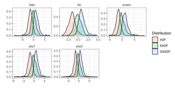
# Apply the critical values to actual data
rsim_data <- radf(sim_data, minw = 20)
autoplot(rsim_data, cv = wb2)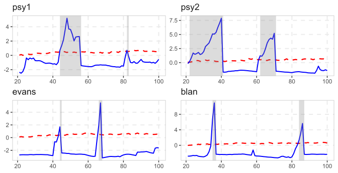
See also
radf_wb_cv for the Harvey et al. (2016) wild bootstrap, radf_mc_cv for Monte Carlo critical values and radf_sb_cv for sieve bootstrap critical values.
Other critical values: radf_common_cv(), radf_mc_cv(), radf_recovery_cv(), radf_sb_cv(), radf_sbz_cv(), radf_sign_cv(), radf_sign_dm_cv(), radf_tt_cv(), radf_wb_cv()
References
Phillips, P. C., & Shi, S. (2020). Real time monitoring of asset markets: Bubbles and crises. In Handbook of Statistics (Vol. 42, pp. 61-80). Elsevier.
Phillips, P. C. B., Shi, S., & Yu, J. (2015). Testing for Multiple Bubbles: Historical Episodes of Exuberance and Collapse in the S&P 500. International Economic Review, 56(4), 1043-1078. 10.1111/iere.12132