 exuber
Recursive Augmented Dickey-Fuller
Monte Carlo Critical Values
Also: radf_mc_distr
radf_mc_cv radf_mc_cv(n, minw = NULL, nrep = 1000L, seed = NULL, lag = 0)
radf_mc_distr(n, minw = NULL, nrep = 1000L, seed = NULL, lag = 0)radf_mc_cv computes Monte Carlo critical values for the recursive unit root tests. radf_mc_distr computes the simulated distribution.
Arguments
| n | A positive integer. The sample size. |
| minw | A positive integer. The minimum window size (default = , where T denotes the sample size). |
| nrep | A positive integer. The number of Monte Carlo simulations. |
| seed | An object specifying if and how the random number generator (rng)
should be initialized. It is either NULL or an integer, which is passed to
set.seed before the simulation. If you set it, the value is saved as the
"seed" attribute of the returned value. The default, NULL, leaves the state of
the rng unchanged and returns .Random.seed as the "seed" attribute. Results are
reproducible across the parallel and the non-parallel option when you use the
same seed. |
| lag | A non-negative integer. Number of lags in the auxiliary
regression, as in radf. |
Value
For radf_mc_cv, a list with the critical values for the ADF, BADF, BSADF and GSADF test statistics. For radf_mc_distr, a list with the ADF, SADF and GSADF distributions.
Examples
These examples are copied from the package's own documentation and are run by R CMD check on every release.
The printed output (after #>) and the plots were produced by running them against the current package source.
# Default minimum window
mc <- radf_mc_cv(n = 100)

tidy(mc)
#> # A tibble: 3 × 4
#>   sig       adf  sadf gsadf
#>   <fct>   <dbl> <dbl> <dbl>
#> 1 90    -0.411  0.996  1.68
#> 2 95    -0.0711 1.33   1.97
#> 3 99     0.746  1.95   2.51

# Change the minimum window and the number of simulations
mc2 <- radf_mc_cv(n = 100, nrep = 600, minw = 20)

tidy(mc2)
#> # A tibble: 3 × 4
#>   sig       adf  sadf gsadf
#>   <fct>   <dbl> <dbl> <dbl>
#> 1 90    -0.274   1.05  1.63
#> 2 95    -0.0125  1.35  1.97
#> 3 99     0.629   1.99  2.47

mdist <- radf_mc_distr(n = 100, nrep = 1000)

autoplot(mdist)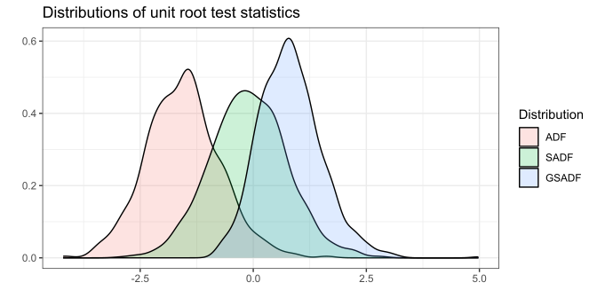
# Apply the critical values to actual data
rsim_data <- radf(sim_data, minw = 20)
autoplot(rsim_data, cv = mc2)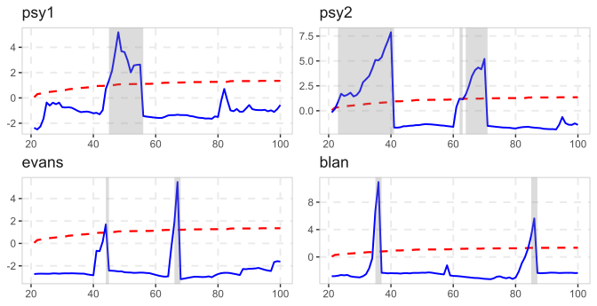
See also
radf_wb_cv for wild bootstrap critical values and radf_sb_cv for sieve bootstrap critical values
Other critical values: radf_common_cv(), radf_recovery_cv(), radf_sb_cv(), radf_sbz_cv(), radf_sign_cv(), radf_sign_dm_cv(), radf_tt_cv(), radf_wb_cv(), radf_wb_ps_cv()