Recursive Augmented Dickey-Fuller

Plotting radf models

Also: autoplot2.radf_obj, shade

autoplot.radf_obj

autoplot(
  object,
  cv = NULL,
  sig_lvl = 95,
  option = c("gsadf", "sadf"),
  min_duration = 0L,
  select_series = NULL,
  nonrejected = FALSE,
  shade_opt = shade(),
  trunc = TRUE,
  include_negative = "DEPRECATED",
  ...
)

autoplot2(
  object,
  cv = NULL,
  sig_lvl = 95,
  option = c("gsadf", "sadf"),
  min_duration = 0L,
  select_series = NULL,
  nonrejected = FALSE,
  trunc = TRUE,
  shade_opt = shade(),
  ...
)

shade(
  fill = "grey55",
  fill_negative = fill,
  fill_ongoing = NULL,
  opacity = 0.3,
  ...
)

autoplot.radf_obj takes a radf_obj and a radf_cv and returns a faceted ggplot object. shade is used as an input to shade_opt. It modifies the geom_rect layer that marks the exuberance periods.

Arguments

object	An object of class `obj`.
cv	An object of class `cv`.
sig_lvl	Significance level. It could be one of 90, 95 or 99.
option	Whether to apply the "gsadf" or the "sadf" methodology (default = "gsadf"). Unlike `datestamp`, this function does not support `"svadf"`, because that option has no critical-value band to shade.
min_duration	The minimum duration of an explosive period for it to be reported (default = 0).
select_series	A vector of column names or numbers that specifies the series to plot. The order of the series does not change the order used in the plot.
nonrejected	If TRUE, plot all series, whether or not they reject the null at the 5 percent significance level.
shade_opt	Shading options, typically set using `shade` function.
trunc	Whether to remove the period of the minimum window from the plot (default = TRUE).
include_negative	Argument name is deprecated and substituted with `nonrejected`.
...	Further arguments passed to `ggplot2::facet_wrap` and `ggplot2::geom_rect` for `shade`.
fill	The shade color for the exuberance periods with a positive signal.
fill_negative	The shade color for the exuberance periods with a negative signal, that is, from series that do not reject the null hypothesis.
fill_ongoing	The shade color for the exuberance periods that are ongoing.
opacity	The opacity of the shade color (alpha).

Value

A ggplot

Examples

These examples are copied from the package's own documentation and are run by R CMD check on every release. The printed output (after #>) and the plots were produced by running them against the current package source.

rsim_data <- radf(sim_data_wdate)
#> Using `date` as index variable.

autoplot(rsim_data)
#> Using precomputed critical values for `cv`.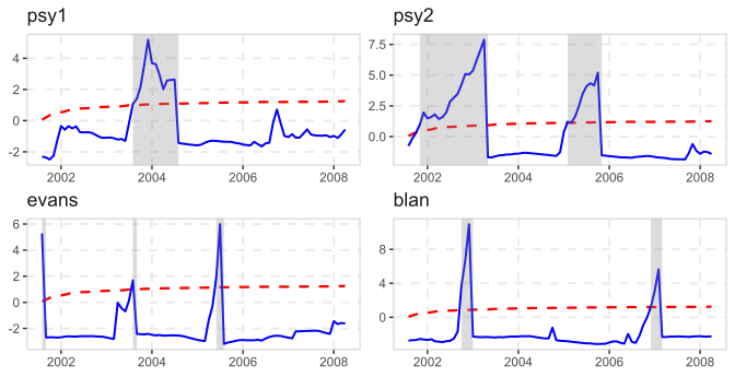

# Modify facet_wrap options through ellipsis
autoplot(rsim_data, scales = "free_y", dir = "v")
#> Using precomputed critical values for `cv`.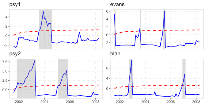

# Modify the shading options
autoplot(rsim_data, shade_opt = shade(fill = "pink", opacity = 0.5))
#> Using precomputed critical values for `cv`.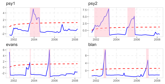

# Allow for nonrejected series to be plotted
autoplot(rsim_data, nonrejected = TRUE)
#> Using precomputed critical values for `cv`.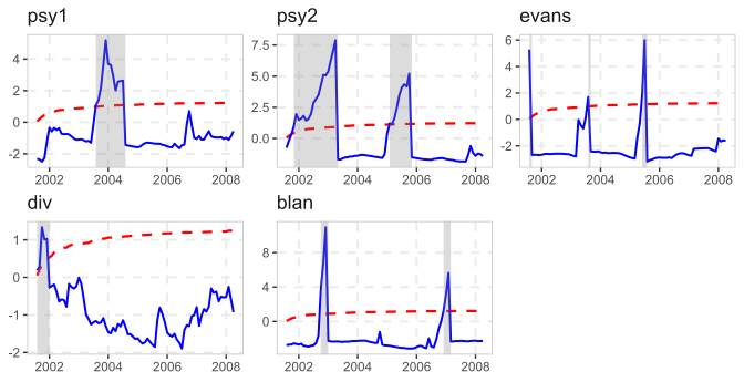

# Remove the shading completely (2 ways)
autoplot(rsim_data, shade_opt = NULL)
#> Using precomputed critical values for `cv`.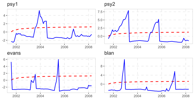

autoplot(rsim_data, shade_opt = shade(opacity = 0))
#> Using precomputed critical values for `cv`.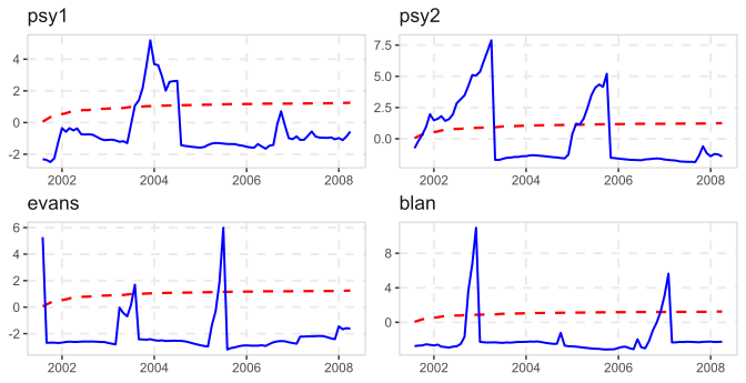

# Plot only the series with the shading options
autoplot2(rsim_data)
#> Using precomputed critical values for `cv`.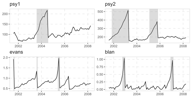

autoplot2(rsim_data, trunc = FALSE) # keep the minw period
#> Using precomputed critical values for `cv`.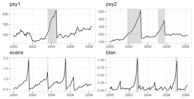

# We will need ggplot2 from here on out
library(ggplot2)

# Change (overwrite) color, size or linetype
autoplot(rsim_data) +
  scale_color_manual(values = c("black", "black")) +
  scale_linewidth_manual(values = c(0.9, 1)) +
  scale_linetype_manual(values = c("solid", "solid"))
#> Using precomputed critical values for `cv`.
#> Scale for colour is already present.
#> Adding another scale for colour, which will replace the existing scale.
#> Scale for linewidth is already present.
#> Adding another scale for linewidth, which will replace the existing scale.
#> Scale for linetype is already present.
#> Adding another scale for linetype, which will replace the existing scale.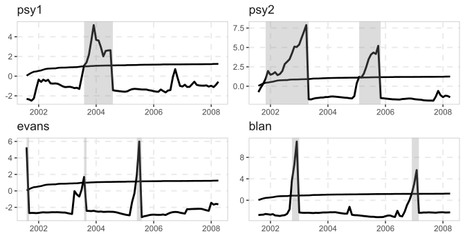

# Change names through labeller (first way)
custom_labels <- c("psy1" = "new_name_for_psy1", "psy2" = "new_name_for_psy2")
autoplot(rsim_data, labeller = labeller(.default = label_value, id = as_labeller(custom_labels)))
#> Using precomputed critical values for `cv`.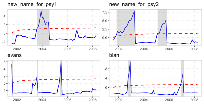

# Change names through labeller (second way)
custom_labels2 <- series_names(rsim_data)
names(custom_labels2) <- custom_labels2
custom_labels2[c(3, 5)] <- c("Evans", "Blanchard")
autoplot(rsim_data, labeller = labeller(id = custom_labels2))
#> Using precomputed critical values for `cv`.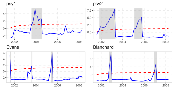

# Or change names before plotting
series_names(rsim_data) <- LETTERS[1:5]
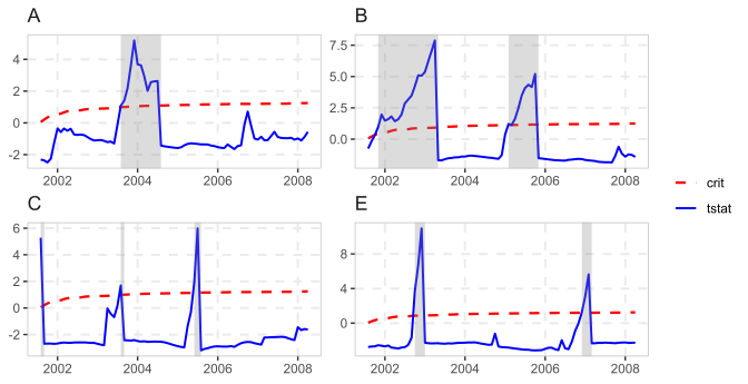
autoplot(rsim_data)
#> Using precomputed critical values for `cv`.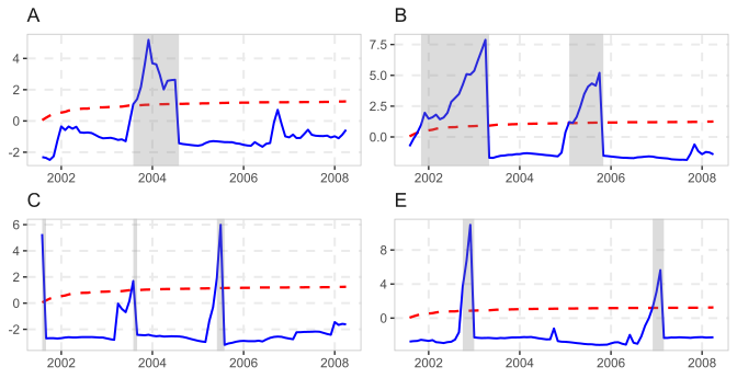

# Change Theme options
autoplot(rsim_data) +
  theme(legend.position = "right")
#> Using precomputed critical values for `cv`.