 exuber
Dating procedures
SSR/BIC Bubble Dating (Harvey, Leybourne & Sollis 2017)
dating_hls
Replication record →
dating_hls(data, trim = 0.05)dating_hls dates a single bubble episode by fitting four candidate regime-dummy regressions of Delta y_t on y_{t-1} (unit-root-to-end, unit-root-bubble-unit-root, unit-root-bubble-collapse and unit-root-bubble-collapse-unit-root). It fits each by minimizing the residual sum of squares over candidate break fractions and selects among them by BIC.
Arguments
| data | A univariate or multivariate numeric time series object, a numeric
vector or matrix, or a data.frame. A column may have leading or trailing
NA values, which describes an unbalanced panel in which series enter or
exit the sample at different times. Those periods are filled with NA in
badf and bsadf and excluded from the adf, sadf and
gsadf of that series. Interior NA values (a gap in the middle of
a series) are not supported. When any series is padded in this way, the panel
statistics (bsadf_panel and gsadf_panel) are not available, and
the function returns NA for them with a warning. |
| trim | Minimum fraction of the (differenced) sample required in every regime (default 0.05, following the choice of Harvey, Leybourne & Sollis in their empirical application. Their simulations use 0.1). |
Value
An object of class dating_hls_obj: a list with the selected model (model, one of 1:4), its breakpoint date or dates (origination, collapse and recovery, with NA for the breakpoints that the selected model does not have), and the BIC value of every candidate model (bic, which shows how close the selection was).
Details
datestamp uses threshold crossing on the recursive BSADF statistic, and dating_pdc uses a fixed structure of three or four regimes with breaks that are estimated sequentially and not jointly. This function searches for the breakpoints jointly within each of four candidate regime structures and lets the BIC pick the structure itself. It can therefore distinguish a bubble that collapses to a new stationary regime (Model 3) from a bubble that fully reverts to a unit root (Model 4) and from a bubble that is still ongoing at the end of the sample (Model 1), which the fixed regime count of dating_pdc cannot. The cost is a joint grid search, in place of the sequential scan of dating_pdc that finds one break at a time.
Status
[Experimental]
Examples
These examples are copied from the package's own documentation and are run by R CMD check on every release.
The printed output (after #>) and the plots were produced by running them against the current package source.
res <- dating_hls(sim_data$psy1, trim = 0.05)
print(res)
#>
#> ── dating_hls (n = 100, trim = 0.05) ───────────────────────────────────────────
#>
#>    series  model  origination  collapse  recovery
#>   series1      4           41        55        62

# Plot the series with the selected model's breakpoint(s) overlaid
autoplot(res)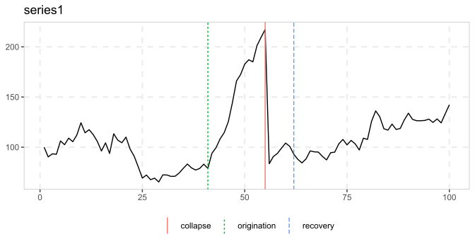
# A whole panel at once, with one subplot for each series
autoplot(dating_hls(sim_data, trim = 0.05))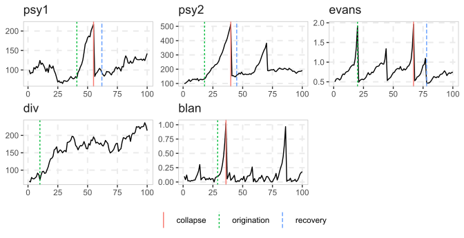
See also
dating_pdc for the cheaper sequential-splitting alternative that this function complements, and datestamp for the original threshold-crossing rule of PSY.
Other dating: dating_hlw(), dating_knp(), dating_pdc(), radf_recovery(), rootstamp()
References
Harvey, D. I., Leybourne, S. J., & Sollis, R. (2017). Improving the accuracy of asset price bubble start and end date estimators. Journal of Empirical Finance, 40, 121-138.