 exuber
Dating procedures
Sequential Sample-Splitting Bubble Dating (PDC/KS)
dating_pdc
Replication record →
dating_pdc(
  data,
  regimes = 3L,
  trim = 0.05,
  type = c("ols", "wls"),
  kernel = c("gaussian", "uniform"),
  h = NULL
)
dating_pdc dates a single bubble episode with the sequential sample-splitting method of Pang, Du & Chong (2021) and its four-regime extension by Kurozumi & Skrobotov (2023). The regime structure is fixed: a unit root, an explosive regime, a stationary collapse and, optionally, a final unit-root recovery regime. The breakpoints are estimated one at a time. Each is a closed-form residual-sum-of-squares minimization over a no-intercept AR(1) model, computed in time with cumulative sums.
Arguments
| data | A univariate or multivariate numeric time series object, a numeric
vector or matrix, or a data.frame. A column may have leading or trailing
NA values, which describes an unbalanced panel in which series enter or
exit the sample at different times. Those periods are filled with NA in
badf and bsadf and excluded from the adf, sadf and
gsadf of that series. Interior NA values (a gap in the middle of
a series) are not supported. When any series is padded in this way, the panel
statistics (bsadf_panel and gsadf_panel) are not available, and
the function returns NA for them with a warning. |
| regimes | Either 3 (PDC: unit root, explosive, stationary collapse)
or 4 (KS: adds a final unit-root recovery regime after the collapse). |
| trim | Minimum fraction of the (differenced) sample required on either side of each breakpoint search (default 0.05, as in the empirical application of KS. PDC use 0.05 to 0.1 in their simulations). |
| type | "ols" (default) for the plain homoskedastic estimator, or
"wls" for the volatility-corrected two-step estimator of Kurozumi &
Skrobotov (2023). |
| kernel | Kernel for the spot-volatility estimator when type = "wls",
"gaussian" (default) or "uniform". It is ignored when
type = "ols". |
| h | Bandwidth for the spot-volatility estimator when type = "wls".
The default is leave-one-out cross-validation. It is ignored when
type = "ols". |
Value
An object of class dating_pdc_obj. It is a data.frame with one row for each series and the columns origination, collapse and, if regimes = 4, recovery, which give the estimated break dates (or observation indices, if no date index is available). It has its own print() and autoplot() methods.
Details
datestamp finds where the recursive BSADF statistic crosses a critical value. This function instead fits an explicit regime-switching model directly to the series, and it needs no critical values. PDC prove that the collapse date is identified first, because its effect on the residual sum of squares dominates that of the origination date. This justifies estimating the breaks sequentially and not jointly. The alternative of Harvey, Leybourne & Sollis (2017) selects among models by BIC and fits them jointly, and it is not implemented here (see the package's enhancement notes for the cost and benefit considerations).
type = "wls" adds the correction of Kurozumi & Skrobotov (2023) for time-varying volatility. The function first fits the plain ("ols") model and collects its fitted residuals for each regime. It then smooths their squares nonparametrically, with the same Nadaraya-Watson kernel and leave-one-out bandwidth estimator that exuber already uses in radf_sbz_cv and radf_kp. Finally it reruns the same sequential break search with each squared term weighted by the inverse of the estimated spot variance. This needs no new critical-value theory. Like the OLS version, it is a point estimate and not a threshold-crossing test.
Status
[Experimental]
Examples
These examples are copied from the package's own documentation and are run by R CMD check on every release.
The printed output (after #>) and the plots were produced by running them against the current package source.
# The unit-root, explosive, collapse and recovery process of sim_ps1() is the
# regime structure that dating_pdc() fits (true breaks at 40, 60 and 70)
y <- sim_ps1(n = 100, seed = 1)
res <- dating_pdc(y, regimes = 3L, trim = 0.05)
print(res)
#>
#> ── dating_pdc (n = 100, regimes = 3, type = ols) ───────────────────────────────
#>
#>    series  origination  collapse
#>   series1           38        59
autoplot(res)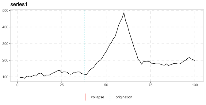
# Four-regime extension, which adds a post-collapse recovery breakpoint
res4 <- dating_pdc(y, regimes = 4L, trim = 0.05)
autoplot(res4)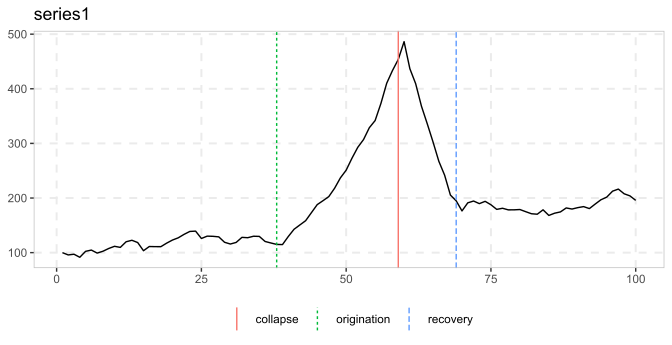
# Volatility-weighted (WLS) variant, robust to time-varying volatility
y_vol <- sim_ps1(n = 100, seed = 1, e = sim_vol_break(99))
autoplot(dating_pdc(y_vol, type = "wls"))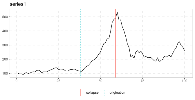
See also
datestamp for the threshold-crossing alternative of PSY.
Other dating: dating_hls(), dating_hlw(), dating_knp(), radf_recovery(), rootstamp()
References
Pang, T., Du, L., & Chong, T. T. L. (2021). Estimating multiple breaks in the bubble regime with SSR minimization. Journal of Management Science and Engineering.
Kurozumi, E., & Skrobotov, A. (2023). Bubble dating: a sequential testing approach.
Kurozumi, E., & Skrobotov, A. (2023). Improving the accuracy of bubble date estimators under time-varying volatility. arXiv:2306.02977.