 exuber
Simulation
Simulation of dividends
sim_div sim_div(
n,
mu,
sigma,
r = 0.05,
log = FALSE,
output = c("pf", "d"),
seed = NULL
)Simulate (log) dividends from a random walk with drift.
Arguments
| n | A positive integer specifying the length of the simulated output series. |
| mu | A scalar indicating the drift. |
| sigma | A positive scalar indicating the standard deviation of the innovations. |
| r | A positive value indicating the discount factor. |
| log | Logical. If true dividends follow a lognormal distribution. |
| output | A character string giving the fundamental price("pf") or
dividend series("d"). Default is pf. |
| seed | An object specifying if and how the random number generator (rng)
should be initialized. It is either NULL or an integer, which is passed to
set.seed before the simulation. If you set it, the value is saved as the
"seed" attribute of the returned value. The default, NULL, leaves the state of
the rng unchanged and returns .Random.seed as the "seed" attribute. Results are
reproducible across the parallel and the non-parallel option when you use the
same seed. |
Value
A numeric vector of length n.
Details
If log is set to FALSE (default value) dividends follow:
where . The default parameters are , and (the initial value of the dividend sequence). The above equation can be solved to yield the fundamental price:
If log is set to TRUE then dividends follow a lognormal distribution or log(dividends) follow:
where . Default parameters are , . The fundamental price in this case is:
where . All default parameter values are those suggested by West (1988).
Examples
These examples are copied from the package's own documentation and are run by R CMD check on every release.
The printed output (after #>) and the plots were produced by running them against the current package source.
# Price is the sum of the bubble and fundamental components
# 20 is the scaling factor
pf <- sim_div(100, r = 0.05, output = "pf", seed = 123)
pb <- sim_evans(100, r = 0.05, seed = 123)
p <- pf + 20 * pb

autoplot(p)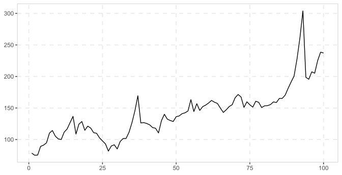
References
West, K. D. (1988). Dividend innovations and stock price volatility. Econometrica: Journal of the Econometric Society, p. 37-61.