 exuber
Simulation
Simulate CIR-type stochastic-volatility innovations
sim_vol_cir sim_vol_cir(
n,
kappa = 0.03,
theta = 0.25,
xi = 0.1,
sigma0_sq = theta,
seed = NULL
)Generates shocks driven by a Cox-Ingersoll-Ross (square-root) stochastic variance process, discretized with the Euler-Maruyama scheme, for use as sim_psy1(..., e = sim_vol_cir(...)).
Arguments
| n | Number of innovations to generate. |
| kappa, theta, xi | Positive CIR parameters (speed of mean reversion, long-run variance and volatility of volatility). |
| sigma0_sq | Non-negative starting variance. Defaults to theta. |
| seed | An object specifying if and how the random number generator (rng)
should be initialized. It is either NULL or an integer, which is passed to
set.seed before the simulation. If you set it, the value is saved as the
"seed" attribute of the returned value. The default, NULL, leaves the state of
the rng unchanged and returns .Random.seed as the "seed" attribute. Results are
reproducible across the parallel and the non-parallel option when you use the
same seed. |
Value
A numeric vector of length n.
Details
discretized over n steps of r in . The variance is reflected at zero if a step would take it negative. The default parameters (, , ) match the robustness design of Harvey, Leybourne & Zu (2019), which is "representative of Bollerslev and Zhou (2002)".
Examples
These examples are copied from the package's own documentation and are run by R CMD check on every release.
The printed output (after #>) and the plots were produced by running them against the current package source.
sim_vol_cir(199, seed = 1) %>%
  autoplot()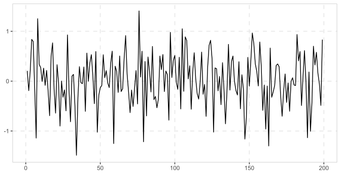
See also
References
Harvey, D.I., Leybourne, S.J. & Zu, Y. (2019). "Testing explosive bubbles with time-varying volatility." Econometric Reviews, 38(10), 1131-1151.