 exuber
Simulation
Simulation of a single-bubble process with multiple forms of collapse regime
sim_ps1 sim_ps1(
n,
te = 0.4 * n,
tf = te + 0.2 * n,
tr = tf + 0.1 * n,
c = 1,
c1 = 1,
c2 = 1,
eta = 0.6,
alpha = 0.6,
beta = 0.5,
sigma = 6.79,
seed = NULL,
e = NULL
)The process differs from the sim_psy1 model in three respects (Phillips and Shi 2018). First, it includes an asymptotically negligible drift in the martingale path during normal periods. Second, the collapse is modeled directly as a transient mildly integrated process that covers an explicit period of market collapse. Third, it introduces a market recovery date to capture the return to normal market behavior. Three forms of collapse are available:
-
sudden:withbeta = 0.1andtr = tf + 0.01*n -
disturbing:withbeta = 0.5andtr = tf + 0.1*n -
smooth:withbeta = 0.9andtr = tf + 0.2*n
To set the duration of the collapse period through tr = tf + 0.2n, you must also provide tf.
Arguments
| n | A positive integer specifying the length of the simulated output series. |
| te | A scalar in (0, tf) specifying the observation in which the bubble originates. |
| tf | A scalar in (te, n) specifying the observation in which the bubble collapses. |
| tr | A scalar in (tf, n) specifying the observation in which market recovers |
| c | A positive scalar determining the drift in the normal market periods. |
| c1 | A positive scalar determining the autoregressive coefficient in the explosive regime. |
| c2 | A positive scalar determining the autoregressive coefficient in the collapse regime. |
| eta | A positive scalar (>0.5) determining the drift in the normal market periods. |
| alpha | A positive scalar in (0, 1) determining the autoregressive coefficient in the bubble period. |
| beta | A positive scalar in (0, 1) determining the autoregressive coefficient in the collapse period. |
| sigma | A positive scalar indicating the standard deviation of the innovations. |
| seed | An object specifying if and how the random number generator (rng)
should be initialized. It is either NULL or an integer, which is passed to
set.seed before the simulation. If you set it, the value is saved as the
"seed" attribute of the returned value. The default, NULL, leaves the state of
the rng unchanged and returns .Random.seed as the "seed" attribute. Results are
reproducible across the parallel and the non-parallel option when you use the
same seed. |
| e | An optional numeric vector of length n - 1 with innovations to
use in place of rnorm(n - 1, sd = sigma). It lets the plain PSY equation
above be driven by a shock sequence that is non-Gaussian, heteroskedastic or
dependent instead of i.i.d. Gaussian noise. The generators sim_innov
(heavy-tailed or skewed), sim_vol_break (permanent volatility
break), sim_vol_garch (GARCH/TGARCH),
sim_vol_cir and sim_vol_sv (stochastic volatility)
and sim_fi (long memory) produce suitable sequences. The default
NULL reproduces the plain i.i.d. Gaussian process exactly. |
Value
A numeric vector of length n.
Examples
These examples are copied from the package's own documentation and are run by R CMD check on every release.
The printed output (after #>) and the plots were produced by running them against the current package source.
# Disturbing collapse (default)
disturbing <- sim_ps1(100)
autoplot(disturbing)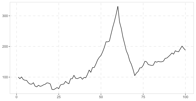
# Sudden collapse
sudden <- sim_ps1(100, te = 40, tf= 60, tr = 61, beta = 0.1)
autoplot(sudden)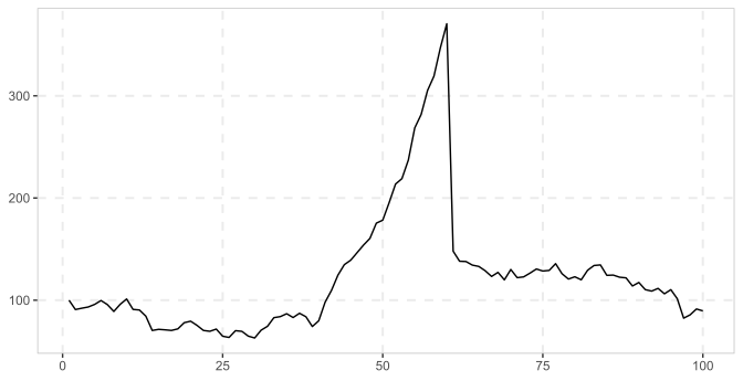
See also
References
Phillips, Peter CB, and Shu-Ping Shi. "Financial bubble implosion and reverse regression." Econometric Theory 34.4 (2018): 705-753.