 exuber
Simulation
Simulation of a deterministic technology-adoption "false bubble" null
sim_falsebubble sim_falsebubble(
n,
t1 = floor(0.3 * n),
t2 = floor(0.7 * n),
kappa = floor((t2 - t1)/2),
shape = c("triangular", "gaussian"),
amplitude = 1,
mu = 0.02,
sigma_d = 0.05,
r = 0.05,
d0 = 0,
seed = NULL
)Simulates the false-bubble process of Chen, Chen, Huang, Li & Zhang (2026): a hump-shaped, deterministic technology-adoption shock embedded in dividend growth. It is engineered so that a Campbell-Shiller present-value fundamental alone, with no bubble component at all, displays a price path that looks locally explosive. It is useful as a null (no-bubble) stress test that differs from a plain random walk.
Arguments
| n | A positive integer specifying the length of the simulated output series. |
| t1 | Adoption (ramp-up start) date, in 1:n. |
| t2 | Maturation (shock end) date, in t1:n. |
| kappa | Peak lag (time from t1 to the hump's peak), in 0:(t2 - t1). |
| shape | "triangular" (default) or "gaussian". |
| amplitude | A positive scalar scaling the hump's peak height. |
| mu | A scalar, the baseline dividend-growth drift. |
| sigma_d | A positive scalar, the dividend-growth innovation standard deviation. |
| r | A positive scalar, the discount rate. |
| d0 | Starting (log) dividend level. |
| seed | An object specifying if and how the random number generator (rng)
should be initialized. It is either NULL or an integer, which is passed to
set.seed before the simulation. If you set it, the value is saved as the
"seed" attribute of the returned value. The default, NULL, leaves the state of
the rng unchanged and returns .Random.seed as the "seed" attribute. Results are
reproducible across the parallel and the non-parallel option when you use the
same seed. |
Value
A numeric vector of length n (the price), with "dividend" and "technology" attributes.
Details
Dividends follow a random walk with drift plus the technology hump: . The hump either rises linearly from t1 to t1 + kappa and then falls linearly to t2 (shape =
"triangular", the worked example of the source, eq. 4), or follows a Gaussian bump centered at t1 + kappa (shape = "gaussian"). Because is deterministic and known in advance, its contribution to the price is an exact forward-looking discounted sum, with , which is added to the fundamental pricing formula that sim_div uses. This is a simplified single-shock reproduction of the mechanism in the source (a deterministic hump gives a hump-shaped fundamental price and no bubble). It does not include the full DOLS and multiple-functional-form robustness machinery of the source.
Examples
These examples are copied from the package's own documentation and are run by R CMD check on every release.
The printed output (after #>) and the plots were produced by running them against the current package source.
sim_falsebubble(200, seed = 123) %>%
  autoplot()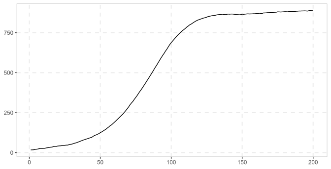
See also
References
Chen, H., Chen, L., Huang, D., Li, Y. & Zhang, Z. (2026). "Technology Fundamentals and False Bubble Detection: Evidence from Dot-Com and AI Episodes." arXiv:2604.25826.