 exuber
Simulation
Simulation of a single-bubble process
sim_psy1 sim_psy1(
n,
te = 0.4 * n,
tf = 0.15 * n + te,
c = 1,
alpha = 0.6,
sigma = 6.79,
seed = NULL,
e = NULL,
shifts = NULL,
coef_noise = NULL,
coef_a = 1
)Generates a time series that switches from a martingale to a mildly explosive process and then back to a martingale.
Arguments
| n | A positive integer specifying the length of the simulated output series. |
| te | A scalar in (0, tf) specifying the observation in which the bubble originates. |
| tf | A scalar in (te, n) specifying the observation in which the bubble collapses. |
| c | A positive scalar determining the autoregressive coefficient in the explosive regime. |
| alpha | A positive scalar in (0, 1) determining the value of the expansion rate in the autoregressive coefficient. |
| sigma | A positive scalar indicating the standard deviation of the innovations. |
| seed | An object specifying if and how the random number generator (rng)
should be initialized. It is either NULL or an integer, which is passed to
set.seed before the simulation. If you set it, the value is saved as the
"seed" attribute of the returned value. The default, NULL, leaves the state of
the rng unchanged and returns .Random.seed as the "seed" attribute. Results are
reproducible across the parallel and the non-parallel option when you use the
same seed. |
| e | An optional numeric vector of length n - 1 with innovations to
use in place of rnorm(n - 1, sd = sigma). It lets the plain PSY equation
above be driven by a shock sequence that is non-Gaussian, heteroskedastic or
dependent instead of i.i.d. Gaussian noise. The generators sim_innov
(heavy-tailed or skewed), sim_vol_break (permanent volatility
break), sim_vol_garch (GARCH/TGARCH),
sim_vol_cir and sim_vol_sv (stochastic volatility)
and sim_fi (long memory) produce suitable sequences. The default
NULL reproduces the plain i.i.d. Gaussian process exactly. |
| shifts | An optional data frame or list with an integer element or column
date (in 2:n) and a numeric element or column size. It adds
a one-period deterministic level shift of magnitude size at each
date, which is the level-shift process of Harvey, Leybourne, Tatlow & Zu
(2025). The default NULL adds no shifts. |
| coef_noise | An optional numeric vector of length n - 1 with zero
mean and unit variance. It perturbs the coefficient of the explosive regime as
delta + coef_a * coef_noise[t] / sqrt(n) instead of the fixed
delta, which gives the stochastically varying explosive coefficient of
Kurozumi & Nishi (2025). The default NULL keeps delta fixed. |
| coef_a | A positive scalar scaling coef_noise. Ignored if
coef_noise is NULL. |
Value
A numeric vector of length n.
Details
The data generating process is described by the following equation:
where the autoregressive coefficient is given by:
with , , and with , dates the origination of the bubble, and dates the collapse of the bubble. During the pre- and post- bubble periods, , is a pure random walk process. During the bubble expansion period becomes a mildly explosive process with expansion rate given by the autoregressive coefficient ; and, finally during the post-bubble period, reverts to a martingale.
For further details see Phillips et al. (2015) p. 1054.
Examples
These examples are copied from the package's own documentation and are run by R CMD check on every release.
The printed output (after #>) and the plots were produced by running them against the current package source.
# 100 periods with bubble origination date 40 and termination date 55
sim_psy1(n = 100, seed = 123) %>%
  autoplot()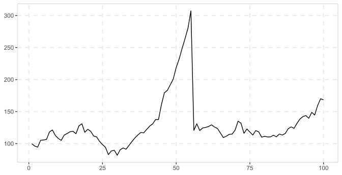
# 200 periods with bubble origination date 80 and termination date 110
sim_psy1(n = 200, seed = 123) %>%
  autoplot()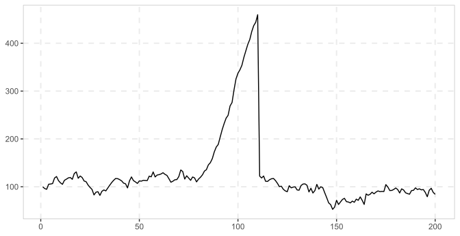
# 200 periods with bubble origination date 100 and termination date 150
sim_psy1(n = 200, te = 100, tf = 150, seed = 123) %>%
  autoplot()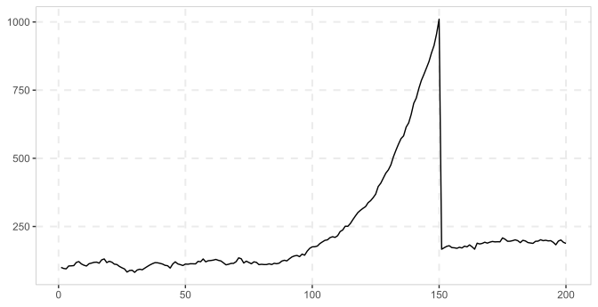
# Same DGP, driven by GARCH(1,1) innovations instead of i.i.d. Gaussian
sim_psy1(n = 200, seed = 123, e = sim_vol_garch(199, seed = 123)) %>%
  autoplot()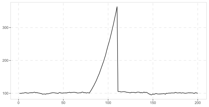
# Same DGP, with two deterministic level shifts
sim_psy1(n = 200, seed = 123, shifts = list(date = c(50, 150), size = c(20, -20))) %>%
  autoplot()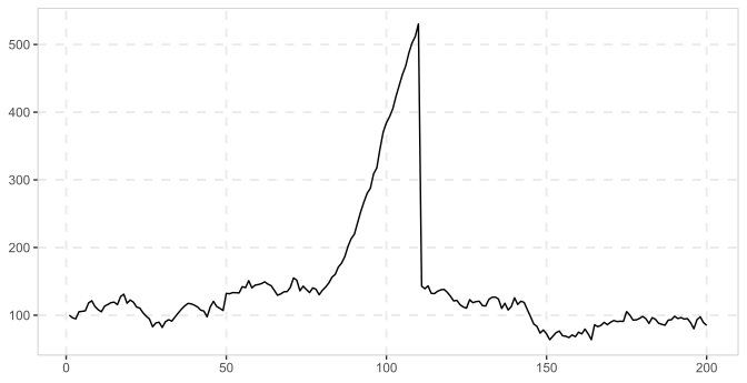
See also
References
Phillips, P. C. B., Shi, S., & Yu, J. (2015). Testing for Multiple Bubbles: Historical Episodes of Exuberance and Collapse in the S&P 500. International Economic Review, 5 6(4), 1043-1078. 10.1111/iere.12132