 exuber
Simulation
Simulation of a mixed causal-noncausal AR(1,1) bubble
sim_mar sim_mar(
n,
phi1 = 0.7,
psi1 = 0.7,
dist = c("cauchy", "t"),
df = 2,
burn = 100,
seed = NULL
)Simulates the mixed causal-noncausal autoregressive (MAR) bubble process of Blasques, Koopman, Mingoli & Telg (2025). Transient, self-terminating local bubbles arise on their own from the noncausal (forward-looking) component. Unlike sim_psy1, no origination or collapse dates are scripted.
Arguments
| n | A positive integer specifying the length of the simulated output series. |
| phi1 | Causal AR coefficient, in (0, 1). |
| psi1 | Noncausal AR coefficient, in (0, 1). |
| dist | Innovation distribution: "cauchy" or "t" (with df degrees of freedom). |
| df | Degrees of freedom if dist = "t". |
| burn | Non-negative burn-in length applied at both ends (see Details). |
| seed | An object specifying if and how the random number generator (rng)
should be initialized. It is either NULL or an integer, which is passed to
set.seed before the simulation. If you set it, the value is saved as the
"seed" attribute of the returned value. The default, NULL, leaves the state of
the rng unchanged and returns .Random.seed as the "seed" attribute. Results are
reproducible across the parallel and the non-parallel option when you use the
same seed. |
Value
A numeric vector of length n.
Details
The function uses the standard two-sided filtering method for MAR processes (Lanne & Saikkonen 2011; Gourieroux & Zakoian 2017). It generates the noncausal component by running backward from a zero boundary burn observations past the end of the sample. It then generates the causal component by running forward from a zero boundary burn observations before the start. Both burn-in windows are then dropped.
Examples
These examples are copied from the package's own documentation and are run by R CMD check on every release.
The printed output (after #>) and the plots were produced by running them against the current package source.
sim_mar(200, seed = 123) %>%
  autoplot()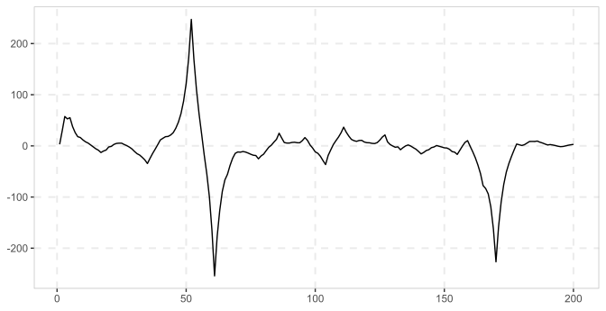
See also
References
Blasques, F., Koopman, S.J., Mingoli, G. & Telg, S. (2025). "A Novel Test for the Presence of Local Explosive Dynamics." JTSA, 46(5), 966-980.