 exuber
Simulation
Simulate innovations with heavy-tailed/skewed marginal distributions
sim_innov sim_innov(
n,
dist = c("normal", "t", "skew_t"),
sigma = 6.79,
df = 5,
xi = 0,
seed = NULL
)Generates a shock sequence for use with the PSY-style mean equations (sim_psy1 and sim_psy2) but with a non-Gaussian marginal distribution. The sequence is standardized to mean 0 and variance sigma^2, so it fits directly into sim_psy1(..., e = sim_innov(...)).
Arguments
| n | Number of innovations to generate. |
| dist | One of "normal", "t", "skew_t". |
| sigma | A positive scalar indicating the standard deviation of the innovations. |
| df | Degrees of freedom for "t"/"skew_t" (> 2). |
| xi | Skewness parameter for "skew_t" (any real; 0 = symmetric). |
| seed | An object specifying if and how the random number generator (rng)
should be initialized. It is either NULL or an integer, which is passed to
set.seed before the simulation. If you set it, the value is saved as the
"seed" attribute of the returned value. The default, NULL, leaves the state of
the rng unchanged and returns .Random.seed as the "seed" attribute. Results are
reproducible across the parallel and the non-parallel option when you use the
same seed. |
Value
A numeric vector of length n.
Details
dist = "t" rescales a Student-t(df) draw to variance 1 before scaling by sigma. This is exact and closed form, because Var(t_df) = df / (df - 2). dist = "skew_t" combines two independent standardized Student-t draws in the manner of Azzalini, delta * abs(T0) + sqrt(1 - delta^2) * T1 with delta = xi / sqrt(1 + xi^2), and then standardizes the result with the closed-form mean and variance of that combination (E|T0| is itself closed form through the Beta function). xi > 0 skews the distribution to the right, xi < 0 skews it to the left, and xi = 0 gives the symmetric t case.
Examples
These examples are copied from the package's own documentation and are run by R CMD check on every release.
The printed output (after #>) and the plots were produced by running them against the current package source.
sim_innov(199, dist = "skew_t", df = 3, xi = -0.75, seed = 1) %>%
  autoplot()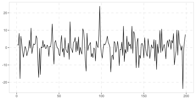
# Feed skew-t innovations into sim_psy1() in place of i.i.d. Gaussian ones
sim_psy1(n = 200, seed = 123, e = sim_innov(199, dist = "skew_t", df = 3, xi = -0.75, seed = 1)) %>%
  autoplot()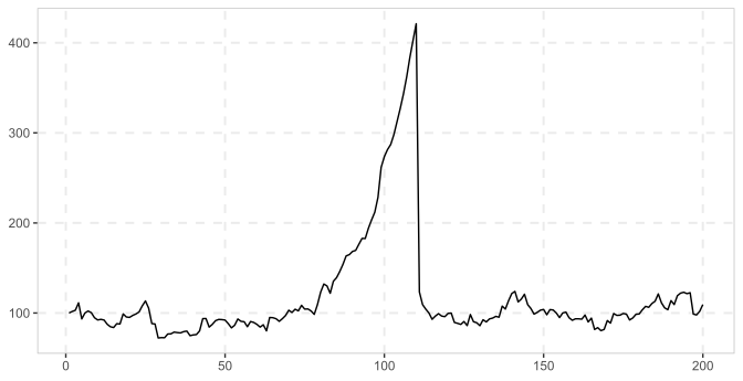
See also
References
Wu, R., Shi, S. & Wu, J. (2025). "Quantile analysis for financial bubble detection and surveillance." JTSA, 46(5), 908-931 (uses N(0,1)/t(3)/skewed-t(3, -0.75)/skewed-t(3, 0.75) innovations in their Monte Carlo design, eq. 6).